COUNT Function

Counts the number of cells (or arguments) that contain a number

What is the COUNT Function?

The COUNT Function[1] is an Excel Statistical function. This function helps count the number of cells that contain a number, as well as the number of arguments that contain numbers. It will also count numbers in any given array. It was introduced in Excel in 2000.

As a financial analyst, it is useful in analyzing data if we wish to keep a count of cells in a given range.

Formula

=COUNT(value1, value2….)

Where:

Value1 (required argument) – The first item or cell reference or range for which we wish to count numbers.

Value2… (optional argument) – We can add up to 255 additional items, cell references, or ranges within which we wish to count numbers.

Remember this function will count only numbers and ignore everything else.

How to use the COUNT Function in Excel?

To understand the uses of this function, let us consider a few examples:

Example 1

Let’s see the results that we get using the data below:

COUNT Function

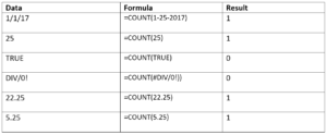
As seen above, the function ignored text or formula errors and counted numbers only.

The results we got in Excel are shown below:

COUNT Function - Example 1

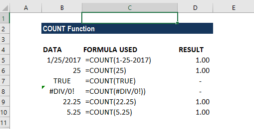
A few observations

Logical values and errors are not counted by this function
As Excel stores dates as a serial number, the function returned 1 count for date.

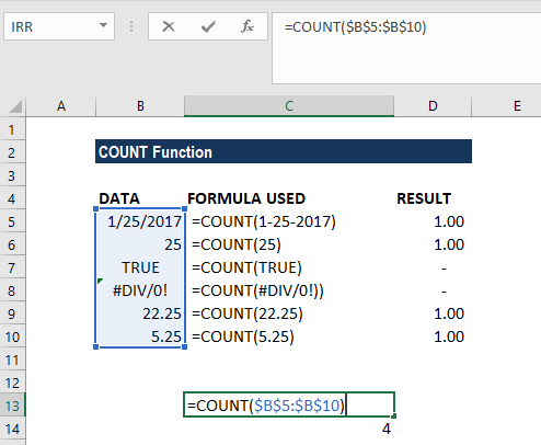
This function can be used for an array. If we use the formula =COUNT(B5:B10), we will get the result 4 as shown below:

COUNT Function - Example 1a

Example 2

Let’s assume we imported data and wish to see the number of cells with numbers in them. The data given are shown below:

COUNT Function - Example 2

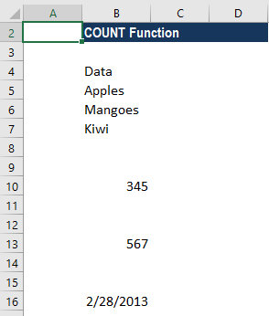
To count the cells with numeric data, we use the formula COUNT(B4:B16).

COUNT Function - Example 2a

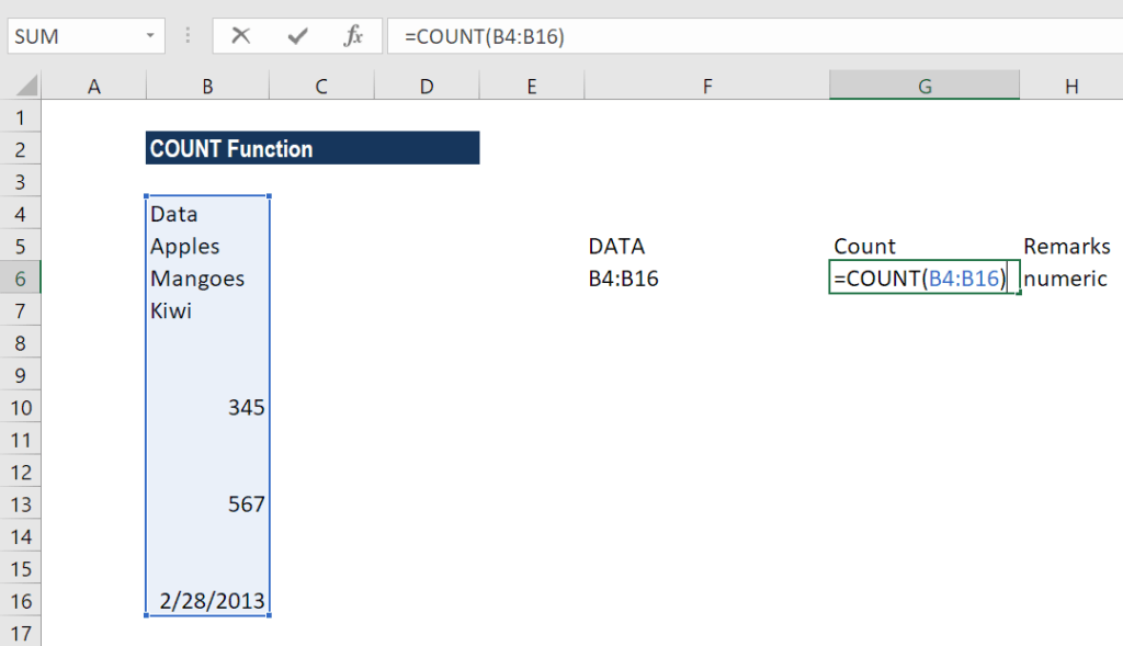
We get 3 as the result, as shown below:

COUNT Function - Example 2b

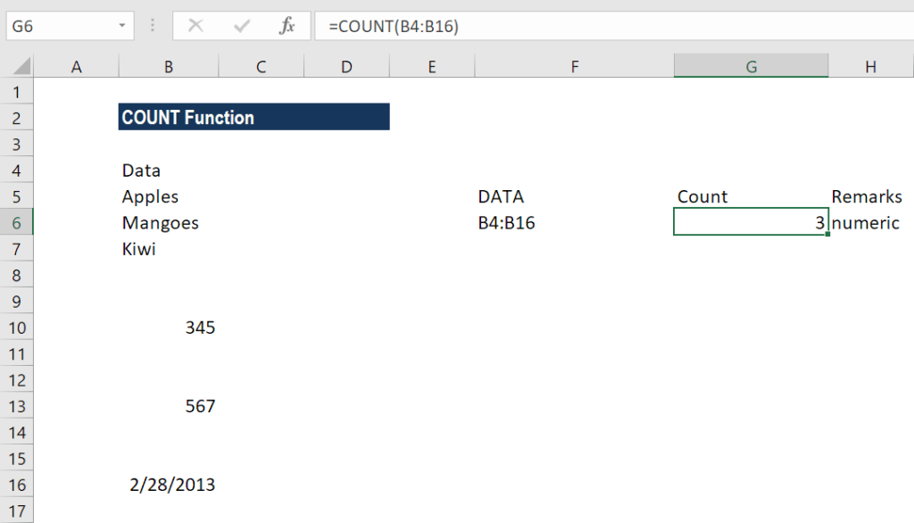
The COUNT function is fully programmed. It counts the number of cells in a range that contain numbers and returns the result as shown above.

Suppose we use the formula COUNT(B5:B17,345). We will get the result below:

COUNT Function - Example 2c

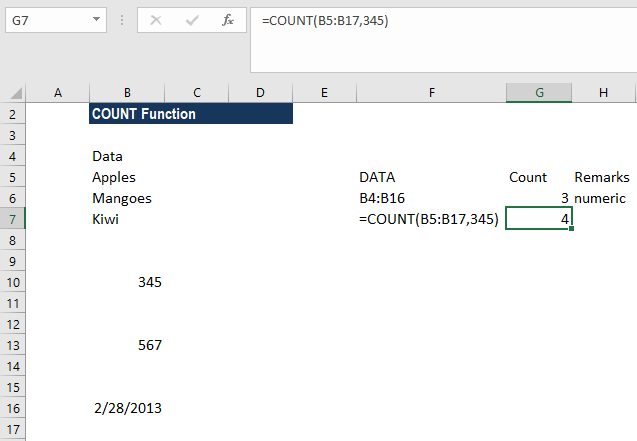
You may be wondering because B10 contains 345 in the given range. So why did the function return 4?

The reason is that in the COUNT function, all values in the formula are put side by side and then all numbers get counted. Therefore, the number “345” has nothing to do with the range. As a result, the formula will add the numbers of the two values in the formula.

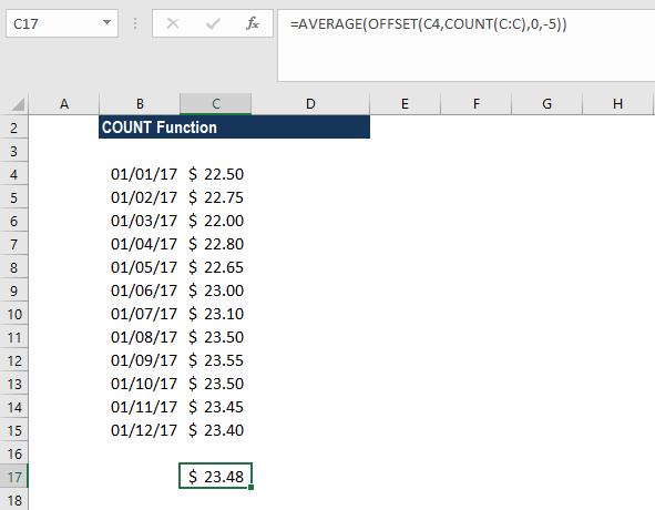
Example 3 – Using COUNT function with the AVERAGE function

Suppose the prices of a certain commodity are given as below:

COUNT Function - Example 3

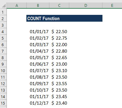
If we wish to find out the average price from January 8 to 12,we can use the AVERAGE function along with the COUNT and OFFSET functions.

The formula to use will be:

COUNT Function - Example 3a

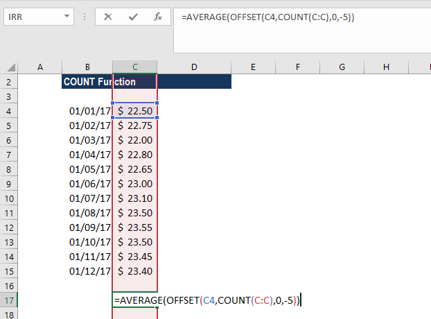
The OFFSET function helped in creating dynamic rectangular ranges. By giving the starting reference B2, we specified the rows and columns the final range would include.

OFFSET will now return a range originating from the last entry in column B. Now the COUNT function is used for all of column B to get the required row offset. It counts only numeric values, so the headings, if any, are automatically ignored.

There are 12 numerical values in column B, so offset would resolve to OFFSET(B2,12,0,-5). With these values, OFFSET starts at B2, offsets 12 rows to B13, then uses -5 to extend the rectangular range up “backward” five rows to create the range B9:B12.

Finally, OFFSET returns the range B9:B12 to the AVERAGE function, which computes the average of values in that range.

COUNT Function - Example 3b

Things to remember

If we wish to count logical values, then we should use the COUNTA function.
The function belongs to the COUNT function family. There are five variants of COUNT functions: COUNT, COUNTA, COUNTBLANK, COUNTIF, and COUNTIFS.
We need to use the COUNTIF function or COUNTIFS function if we want to count only numbers that meet specific criteria.
If we wish to count based on certain criteria, then we should use COUNTIF.
The COUNT function doesn’t count logical values TRUE or FALSE.

Click here to download the sample Excel file

Additional Resources

Thanks for reading CFI’s guide to important Excel functions! By taking the time to learn and master these functions, you’ll significantly speed up your financial analysis. To learn more, check out these additional CFI resources:

Article Sources

COUNT Function