PERCENTRANK Function

What is the PERCENTRANK Function?

The PERCENTRANK Function[1] is categorized under Excel Statistical functions. This function will return the rank of a value in a data set as a percentage. It can be used to evaluate the relative standing of a value within a data set.

In corporate finance, we can use PERCENTRANK to evaluate the standing of a specific test score among all the employee scores on an aptitude test.

The PERCENTILERANK function has been replaced with PERCENTRANK.EXC and PERCENTRANK.INC functions. Although it is still available for backward compatibility, it may not be available in future versions of MS Excel.

Formula

=PERCENTRANK(array,x,[significance])

The PERCENTRANK function uses the following arguments:

1. Array (required argument) – This is the array or range of data that defines relative standing.
2. X (required argument) – The value for which we want to know its rank.
3. Significance (optional argument) – This is a value that identifies the number of significant digits for the returned percentage value. If omitted, PERCENTRANK uses three digits (0.xxx).

How to use the PERCENTRANK Function in Excel?

As a worksheet function, the PERCENTRANK function can be entered as part of a formula in a cell of a worksheet. To understand the uses of the function, let’s consider an example:

Example

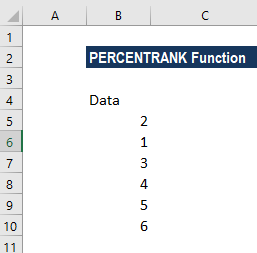
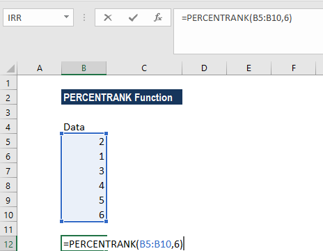
Suppose we are given the following data:

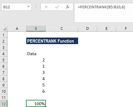
The formula we use is:

We get the results below:

If we provide the formula:

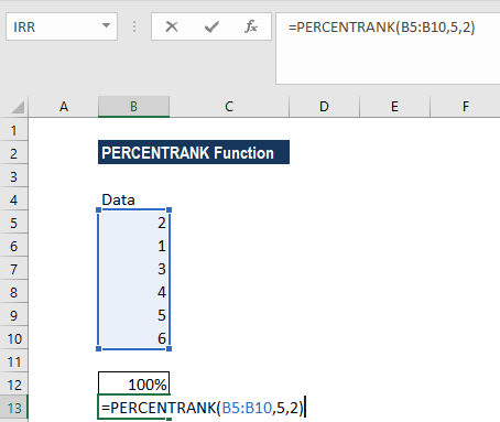
We get the results below:

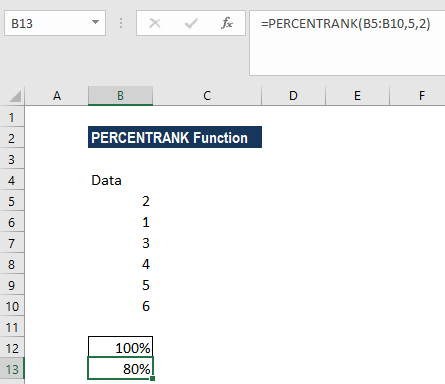
In the formula above, when calculating the PERCENTRANK for the value 5, the function interpolates and the resulting value is rounded down to two significant figures, as specified by the supplied [significance] argument.

Here, we formatted the results to percentage format. If the result of the function is presented as a decimal or shows 0%, it is likely to be due to the formatting of the cell containing the function. It can, therefore, be fixed by formatting the cell as a percentage, with decimal places, if required.

A few notes about the PERCENTRANK Function:

1. #NUM! error – Occurs if either:
   1. If the array is empty
   2. If significance < 1
2. If x does not match one of the values in an array, PERCENTRANK interpolates to return the correct percentage rank.
3. #N/A! error – Occurs if the given value of x is smaller than the minimum, or greater than the maximum, value in the supplied array.

Click here to download the sample Excel file

Additional Resources

Thanks for reading CFI’s guide to the Excel PERCENTRANK function. By taking the time to learn and master these functions, you’ll significantly speed up your financial analysis and Excel modeling. To learn more, check out these additional CFI resources:

• Excel Functions for Finance
• Advanced Excel Formulas Course
• Advanced Excel Formulas You Must Know
• Excel Shortcuts for PC and Mac
• See all Excel resources