AVERAGE Function

How to Calculate AVERAGE in Excel?

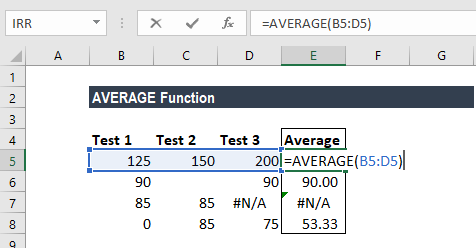
The AVERAGE Function[1] is categorized under Excel Statistical functions. It will return the average value of a given series of numbers in Excel.

The function is used to calculate the arithmetic mean of a given set of arguments in Excel. This guide will show you, step-by-step, how to calculate the average in Excel.

As a financial analyst, the function is useful in finding out the average (mean) of a series of numbers. For example, we can find out the average sales for the last 12 months for a business.

Formula

=AVERAGE(number1, [number2], …)

The function uses the following arguments:

1. Number1 (required argument) – This is the first number of a cell reference or a range for which we want the average.
2. Number2 (optional argument) – They are the additional numbers, cell references or a range for which we want the average. A maximum of 255 numbers is allowed.

How to use AVERAGE Function in Excel?      

To understand the uses of the AVERAGE function, let us consider a few examples:

Example 1 – Average in Excel

Suppose we are given the following data:

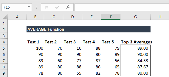
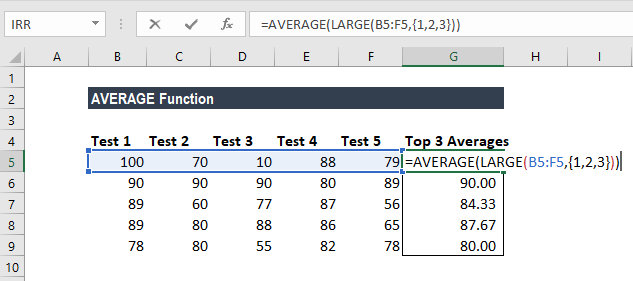
We wish to find out the top 3 scores in the above data set. The formula to use will be:

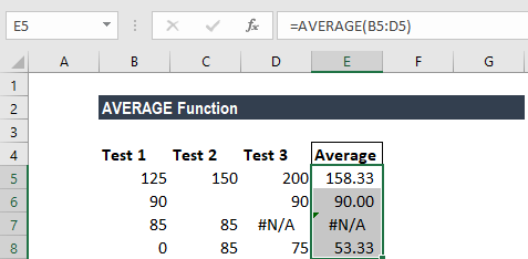
We get the result below:

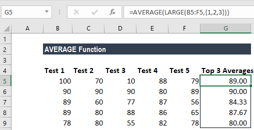
In the above formula, the LARGE function retrieved the top nth values from a set of values. So, we got the top 3 values as we used the array constant {1,2,3} into LARGE for the second argument.

Later, the AVERAGE function returned the average of the values. As the function can automatically handle array results, we don’t need not use Ctrl+Shift+Enter to enter the formula.

Example 2 – Average in Excel

Suppose we are given the data below:

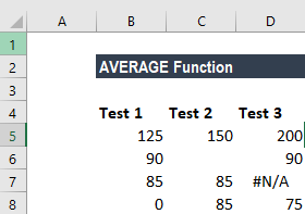
The formula to use is shown below:

We get the following result:

A few notes about the AVERAGE Function

1. The AVERAGE function ignores empty cells.
2. If a range or cell reference argument contains text, logical values, or empty cells, those values are ignored. However, cells with the value zero are included.
3. Arguments that are error values or text that cannot be translated into numbers cause errors in the function.

Click here to download the sample Excel file

Additional Resources

Thanks for reading CFI’s guide to the Excel AVERAGE function. By taking the time to learn and master these functions, you’ll significantly speed up your financial analysis. To learn more, check out these additional CFI resources:

• Free Excel Fundamentals Course
• Advanced Excel Formulas You Must Know
• AVERAGE Function
• AVERAGEA Function
• AVERAGEIFS Function
• See all Excel resources