Index Match Formula

What is INDEX MATCH in Excel?

The INDEX MATCH[1] Formula is the combination of two functions in Excel: INDEX[2] and MATCH[3].

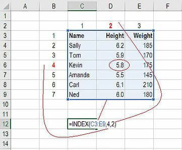
=INDEX() returns the value of a cell in a table based on the column and row number.

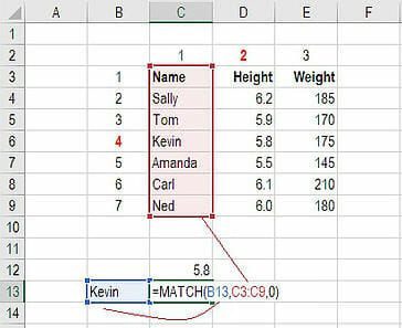
=MATCH() returns the position of a cell in a row or column.

Combined, the two formulas can look up and return the value of a cell in a table based on vertical and horizontal criteria.  For short, this is referred to as just the Index Match function. To see a video tutorial, check out our free Excel Crash Course.

How to Use the INDEX Formula

Below is a table showing people’s names, height, and weight. We want to use the INDEX formula to look up Kevin’s height… here is an example of how to do it.

Follow the steps below:

1. Type “=INDEX(” and select the area of the table, then add a comma
2. Type the row number for Kevin, which is “4,” and add a comma
3. Type the column number for Height, which is “2,” and close the bracket
4. The result is “5.8.”

How to Use the MATCH Formula

Sticking with the same example as above, let’s use MATCH to figure out what row Kevin is in.

Follow the steps below:

1. Type “=MATCH(” and link to the cell containing “Kevin”… the name we want to look up.
2. Select all the cells in the Name column (including the “Name” header).
3. Type zero “0” for an exact match.
4. The result is that Kevin is in row “4.”

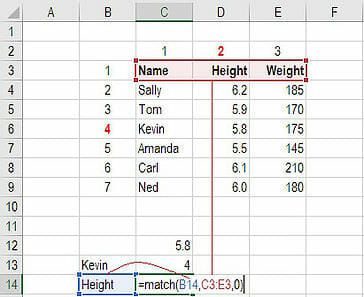
Use MATCH again to figure out what column Height is in.

Follow the steps below:

1. Type “=MATCH(” and link to the cell containing “Height”… the criteria we want to look up.
2. Select all the cells across the top row of the table.
3. Type zero “0” for an exact match.
4. The result is that Height is in column “2.”

How to Combine INDEX and MATCH

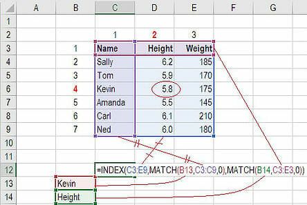
Now, we can take the two MATCH formulas and use them to replace the “4” and the “2” in the original INDEX formula. The result is an INDEX MATCH formula.

Follow the steps below:

1. Cut the MATCH formula for Kevin and replace the “4” with it.
2. Cut the MATCH formula for Height and replace the “2” with it.
3. The result is Kevin’s Height is “5.8.”
4. Congratulations, you now have a dynamic INDEX MATCH formula!

Video Explanation of How to Use Index Match in Excel

Below is a short video tutorial on how to combine the two functions and effectively use Index Match in Excel! Check out more free Excel tutorials on CFI’s YouTube Channel.

Hopefully, the above short video made it even clearer how to use the two functions to dramatically improve your lookup capabilities in Excel.

More Excel Lessons

Thank you for reading this step-by-step guide to using INDEX MATCH in Excel. To continue learning and advancing your skills, these additional CFI resources will be helpful:

• Excel Formulas and Functions List
• Excel Add Months to Date
• Go To Special
• Find and Replace
• IF AND Function in Excel
• See all Excel resources