ISFORMULA Function

What is the ISFORMULA Function?

The ISFORMULA Function[1] is categorized under Excel Information functions. It will test a specified cell to see if it contains a formula. If it does contain a formula, then it will return TRUE. If not, then it will return FALSE.

The ISFORMULA function was introduced in MS Excel 2013. The purpose of the function is to show the formula, if any, contained in the cell.

Formula

=ISFORMULA(reference)

The ISFORMULA function uses the following argument:

1. Reference (required argument) – This is a reference to the cell we wish to test. The reference in the formula can be a cell reference, a formula, or a name that refers to a cell.

How to use the ISFORMULA Function in Excel?

It is a built-in function which can be used as a worksheet function in Excel. To understand the uses of this function, let’s consider a few examples:

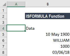
Example 1

Let’s say we are given the data below, and we wish to find out if any formula was used (or not used) in the data.

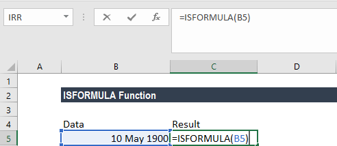
The formula would be ISFORMULA “cellreference” as shown below:

The results would be:

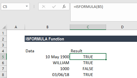
So, the function told us which of the cells contained a formula.

Example 2

Let’s see how this formula can be used with conditional formatting. If we are dealing with large amounts of data and we wish to highlight cells that contain a formula, we can do that using ISFORMULA along with conditional formatting.

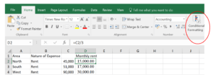
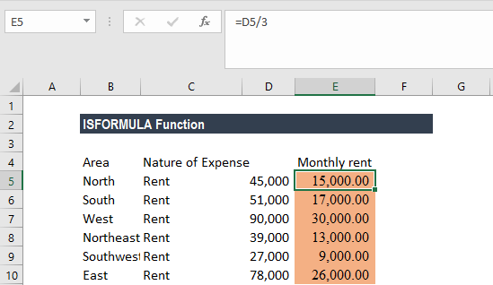
For example, assume we are given the quarterly rent paid and we’ve calculated monthly rent paid in the adjacent column by using the ISFORMULA function.

To apply conditional formatting that will highlight cells with formulas, we need to take the following steps:

1. Select cells D2:D7, with cell D2 as the active cell.
2. After that, click the ‘Conditional Formatting’ command (on the Home tab).

3. Now click on ‘New Rule.’

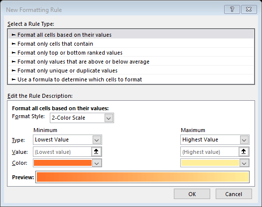
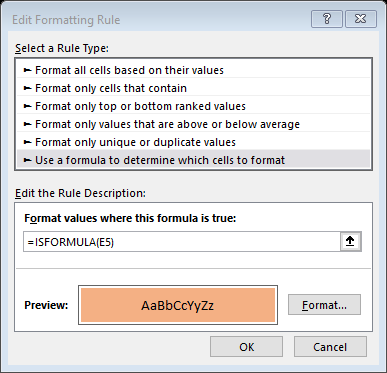
4. Click on ‘Use a Formula’ to determine which cells to format.
5. Enter ISFORMULA formula, referring to the active cell – D2:

=ISFORMULA(D2)

6. Now click on the ‘Format’ button, and select a fill color for the cells with formulas – Peach in this example.

6. Now, click ‘OK’ to close the windows.

Example 3

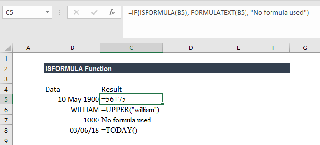
Let’s assume that in Example 1 you don’t wish to get just TRUE or FALSE, but require the formula to return ‘No formula used.’ This can be done by inserting the formula:

=IF(ISFORMULA(B2), FORMULATEXT(B2), “No formula used”)

The results would be:

Example 4

Let’s now see how we can use the FORMULATEXT, ISFORMULA, and TEXTJOIN functions together. Suppose we are given the following data:

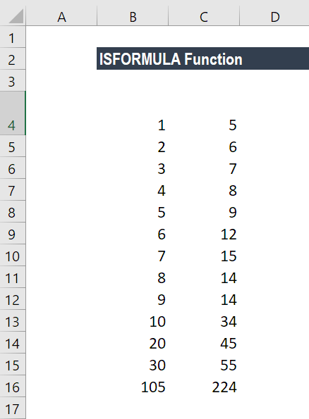
Where row 13 is the sum of all the rows above it.

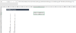
Now, using the formula:

=TEXTJOIN(CHAR(10),TRUE,IF(ISFORMULA(fRange),ADDRESS(ROW(fRange),COLUMN(fRange))&”:”&FORMULATEXT(fRange),””))

We can find out which cells contain a formula. So, FORMULATEXT, ISFORMULA, and TEXTJOIN functions all were used simultaneously.

How does the ISFORMULA Function in Excel work?

1. First, for the (fRange) A1:B13 we provided, we gave ADDRESS(ROW(fRange),COLUMN(fRange)). So, Excel returned an array of cell addresses for the desired range.
2. Next, FORMULATEXT(fRange) returned an array of formulas for that range.
3. The above two formulas were concatenated with a colon, so we got an array that looked like this:

{#N/A,#N/A;#N/A,#N/A;#N/A,#N/A;#N/A,#N/A;#N/A,#N/A;#N/A,#N/A;#N/A,#N/A;#N/A,#N/A;#N/A,#N/A;#N/A,#N/A;#N/A,#N/A;#N/A,#N/A;”$A$13:=SUM(A1:B12)”,”$B$13:=SUM(B1:B12)”}

When we applied the ISFORMULA to it the result was:

{FALSE,FALSE;FALSE,FALSE;FALSE,FALSE;FALSE,FALSE;FALSE,FALSE;FALSE,FALSE;FALSE,FALSE;FALSE,FALSE;FALSE,FALSE;FALSE,FALSE;FALSE,FALSE;FALSE,FALSE;TRUE,TRUE}

Hence, the final array created by the IF function looks like this:

{“”,””;””,””;””,””;””,””;””,””;””,””;””,””;””,””;””,””;””,””;””,””;””,””;”$A$13:=SUM(A1:A12)”,”$B$13:=SUM(B1:B12)”}

When this array was processed by the TEXTJOIN function, it gave a string of formulas with their corresponding cell locations.

So, we got the result as:

A few notes about the ISFORMULA Function

1. #VALUE! error – Occurs when the reference is not a valid data type.
2. Even when a formula entered results in an error, ISFORMULA will return the result as TRUE as long as the cell contains a formula.

Click here to download the sample Excel file

Additional Resources

Thanks for reading CFI’s guide to important Excel functions! By taking the time to learn and master these functions, you’ll significantly speed up your financial analysis. To learn more, check out these additional CFI resources:

• Advanced Excel Formulas You Must Know
• Excel Shortcuts for PC and Mac
• ISNA Function
• ISTEXT Function
• See all Excel resources