Get Certified for
Business Intelligence (BIDA®)
Develop analytical superpowers by learning how to use programming and data analytics tools such as VBA, Python, Tableau, Power BI, Power Query, and more.
A distribution of data in statistics that has discrete values
A discrete distribution is a distribution of data in statistics that has discrete values. Discrete values are countable, finite, non-negative integers, such as 1, 10, 15, etc.

The two types of distributions are:
A discrete distribution, as mentioned earlier, is a distribution of values that are countable whole numbers. On the other hand, a continuous distribution includes values with infinite decimal places. An example of a value on a continuous distribution would be “pi.” Pi is a number with infinite decimal places (3.14159…).
Both distributions relate to probability distributions, which are the foundation of statistical analysis and probability theory.
A probability distribution is a statistical function that is used to show all the possible values and likelihoods of a random variable in a specific range. The range would be bound by maximum and minimum values, but the actual value would depend on numerous factors. There are descriptive statistics used to explain where the expected value may end up. Some of which are:
Discrete distributions also arise in Monte Carlo simulations. A Monte Carlo simulation is a statistical modeling method that identifies the probabilities of different outcomes by running a very large amount of simulations. From Monte Carlo simulations, outcomes with discrete values will produce a discrete distribution for analysis.
Types of discrete probability distributions include:
Consider an example where you are counting the number of people walking into a store in any given hour. The values would need to be countable, finite, non-negative integers. It would not be possible to have 0.5 people walk into a store, and it would not be possible to have a negative amount of people walk into a store. Therefore, the distribution of the values, when represented on a distribution plot, would be discrete.

Observing the above discrete distribution of collected data points, we can see that there were five hours where between one and five people walked into the store. In addition, there were ten hours where between five and nine people walked into the store and so on.
The probability distribution above gives a visual representation of the probability that a certain amount of people would walk into the store at any given hour. Without doing any quantitative analysis, we can observe that there is a high likelihood that between 9 and 17 people will walk into the store at any given hour.
Continuous probability distributions are characterized by having an infinite and uncountable range of possible values. The probabilities of continuous random variables are defined by the area underneath the curve of the probability density function.
The probability density function (PDF) is the likelihood for a continuous random variable to take a particular value by inferring from the sampled information and measuring the area underneath the PDF. Although the absolute likelihood of a random variable taking a particular value is 0 (since there are infinite possible values), the PDF at two different samples is used to infer the likelihood of a random variable.
Consider an example where you wish to calculate the distribution of the height of a certain population. You can gather a sample and measure their heights. However, you will not reach an exact height for any of the measured individuals.
For calculating the distribution of heights, you can recognize that the probability of an individual being exactly 180cm is zero. That is, the probability of measuring an individual having a height of exactly 180cm with infinite precision is zero. However, the probability that an individual has a height that is greater than 180cm can be measured.
In addition, you can calculate the probability that an individual has a height that is lower than 180cm. Therefore, you can use the inferred probabilities to calculate a value for a range, say between 179.9cm and 180.1cm.
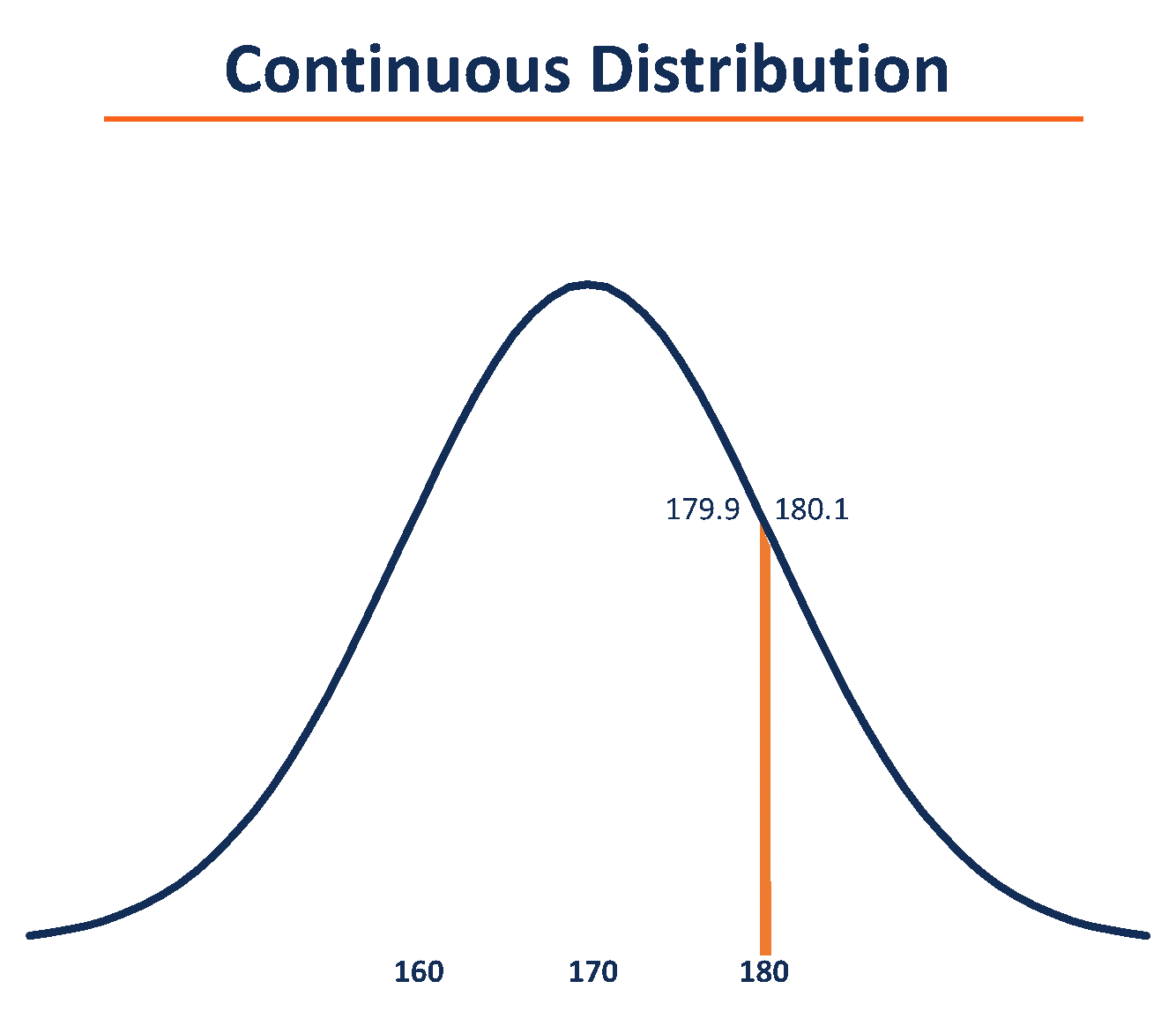
Observing the continuous distribution, it is clear that the mean is 170cm; however, the range of values that can be taken is infinite. Therefore, measuring the probability of any given random variable would require taking the inference between two ranges, as shown above.
CFI offers the Business Intelligence & Data Analyst (BIDA)® certification program for those looking to take their careers to the next level. To keep learning and developing your knowledge base, please explore the additional relevant resources below:


