Get Certified for
Business Intelligence (BIDA®)
Develop analytical superpowers by learning how to use programming and data analytics tools such as VBA, Python, Tableau, Power BI, Power Query, and more.
A close estimate of the actual value of a variable
A ballpark figure is a close estimate of the actual value of a variable. It is typically computed using a simple approximation instead of going about the actual computation process, which is more complicated.

Ballpark figures provide a reasonable estimate when more sophisticated tools, such as spreadsheets, are not available. Many such approximations were widely used before computers became commonplace in the finance industry.
Despite the widespread use of computers nowadays, ballpark calculations remain in use. The simplicity of the estimation methods helps reduce the complexity of the calculation. It helps reduce the chances of introducing an error while doing decimal (floating point) operations, as well as a human error such as inputting an incorrect formula.
In the next sections, we will see examples of ballpark figures as used in different areas of finance, such as time value of money, derivatives, real estate, and more.
The most common example of using a ballpark figure comes from the very basics of finance – the Rule of 72. The rule simply states that to calculate the amount of time it takes for an investment to double is given by the following simple formula:
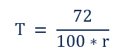
Where:
As the chart below illustrates, the rule of 72 is an excellent estimate when compared to the actual value computed using the NPER function in Excel.
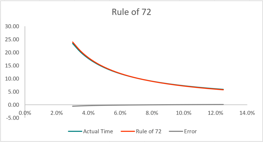
It is important to note that the rule does apply if the investment includes intermediate payments, such as an annuity. It is because as payments increase, the time taken to double the investment falls very fast.
Bonds come with all sorts of metrics associated with them. One such metric is the bond duration. The duration of a bond is the sensitivity of its price to change in the yield to maturity. For the scope of this article, we will only look at how it is computed using a formula compared to an estimate of the duration.
The following formula is used to compute the duration of a simple coupon bond:

Where:
The choice of t and T depends on the day count convention used in valuation. In short, it is very complicated with lots of moving parts. The ballpark estimate for the duration is given by a simpler procedure described below:

Where:
The calculation of market value can be done easily using the PV function in Excel, then plugging the values in the above formula. The figure below summarizes the two methods and their results.

The calculation can be made more precise by reducing the value of ∆y as close to zero as possible or to a satisfactory degree of precision.
The most commonly used discount rate while valuing equities is the Weighted Average Cost of Capital (WACC). The WACC includes many inputs, and some of the inputs are estimated rather than being explicitly calculated. Two such inputs are the beta and the equity risk premium (ERP), which is used to calculate the cost of equity.
There are many ways to determine beta. The explicit approach is to run a regression of stock returns against the market returns. However, it leads to discrepancies in the estimates of beta due to the data used (daily or weekly returns, length of history, etc.). To overcome such a problem, an average or median of comparable company betas from a reliable source is used to arrive at an estimate of the beta.
Similarly, for the ERP, a consensus estimate is used to do the calculations instead of doing the statistical work to compute it from raw data. For example, a number of about 5% is a common ballpark figure for the ERP.
The ideas above are illustrated in a well-cited survey, “Best Practices in Estimating Cost of Capital.”
Derivatives are a broad discipline and offer many techniques to calculate different ballpark figures, some more complex than others. The two techniques listed below show how to calculate the price and implied volatility of close to- or at-the-money call options.
The price of a call option is given using the Black-Scholes formula. However, there is an easier way to calculate the price of the option when it is close-to-the-money. The approximation is based on the Black-Scholes framework, as described below:

Where:

The implied volatility of an option is the value of the volatility parameter implied by the market price of the option. It is important to note in valuing options that all inputs can be observed except volatility, which must be estimated. Hence, the difference between the model price (say from the Black-Scholes model) and the market price is attributable to volatility.
To calculate implied volatility, one needs to use a computer program that would do a trial and error search for the correct value of the implied volatility. However, it is possible to get a ballpark figure for implied volatility of close-to-the-money options using the following formula:

Where:

A similar concept to a ballpark figure is the concept of a back-of-the-envelope calculation. The back-of-the-envelope calculation is the simplified version of the actual calculation that gives a ballpark estimate of the required variable.
A common example of such a calculation is the estimation of the cap rate in the real estate sector. There are elaborate models to determine the cap rate of a property, but it can be estimated in a simple calculation described below:
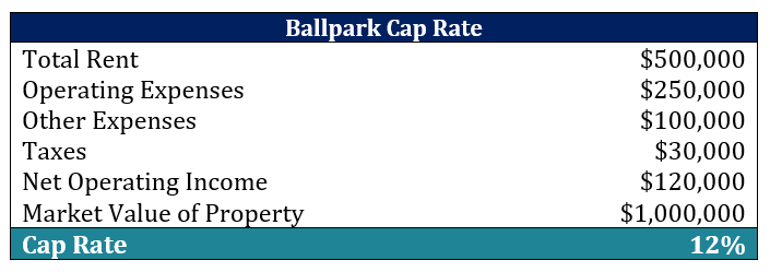
In the above calculation, the cap rate is calculated as:

The net operating income here is derived from basic assumptions and facts about the property. It is a simplistic representation of the more detailed models used in the industry.
Thank you for reading CFI’s guide to Ballpark Figure. To keep advancing your career, the additional CFI resources below will be useful:
Below is a break down of subject weightings in the FMVA® financial analyst program. As you can see there is a heavy focus on financial modeling, finance, Excel, business valuation, budgeting/forecasting, PowerPoint presentations, accounting and business strategy.

A well rounded financial analyst possesses all of the above skills!
CFI is the global institution behind the financial modeling and valuation analyst FMVA® Designation. CFI is on a mission to enable anyone to be a great financial analyst and have a great career path. In order to help you advance your career, CFI has compiled many resources to assist you along the path.
In order to become a great financial analyst, here are some more questions and answers for you to discover:


