Adjusted Present Value (APV)

What is Adjusted Present Value (APV)?

Adjusted Present Value (APV) is used for the valuation of projects and companies. It takes the net present value (NPV), plus the present value of debt financing costs, which include interest tax shields, costs of debt issuance, costs of financial distress, financial subsidies, etc.

So why do we use Adjusted Present Value instead of NPV in evaluating projects with debt financing? To answer this, we first need to understand how financing decisions (debt vs. equity) affect the value of a project. 

Download the Adjusted Present Value Template.

How debt and equity affect the value of a project

The value of a project financed with debt may be higher than that of an all equity-financed project since the cost of capital often decreases with leverage, turning some negative NPV projects into positive ones. Thus, under the NPV rule, a project may be rejected if it is financed with only equity but may be accepted if it is financed with some debt. 

The Adjusted Present Value approach takes into consideration the benefits of raising debt (e.g. interest tax shield), which NPV does not do. As such, APV analysis is preferred in highly leveraged transactions.

APV and financial modeling

In financial modeling, it is common practice to use Net Present Value with the firm’s Weighted Average Cost of Capital as the discount rate, which determines the unlevered value of the firm (its enterprise value) or the unlevered value of a project.

The present value of net debt is deducted to arrive at equity value, if that’s what is desired. See a comparison of equity value vs enterprise value.

To learn more, launch our financial modeling courses!

Adjusted Present Value assumptions

We make the following simplifying assumptions before using the APV approach in the valuation of a project:

1. The project’s risk is equal to the average risks of other projects within the firm, which is also the risk of the firm. In other words, the project in question is a “typical” project that the firm usually takes on. In this case, the relevant discount rate for the project is based on the risk of the firm.
2. Corporate taxes are the only important market imperfection at the level of debt chosen. This means that we focus only on the interest tax shields and ignore the effects generated by the costs of debt issuance and financial distress.
3. All debt is perpetual.

Unlevered cost of capital

The APV method uses unlevered cost of capital to discount free cash flows, as it initially assumes that the project is fully financed by equity.

To find the unlevered cost of capital, we must first find the project’s unlevered beta. Unlevered beta is a measure of the company’s risk relative to that of the market. It is also referred to as “asset beta” because, without leverage, a company’s equity beta is equal to its asset beta.

To retrieve a company’s beta, we can look up the company on financial resource sites such as Bloomberg Terminal or CapIQ.  If the company is not listed, we can find a comparable company that is listed instead.

The unlevered cost of capital is calculated as:

Unlevered cost of capital (rU) = Risk-free rate + beta * (Expected market return – Risk-free rate).

The Adjusted Present Value for valuation

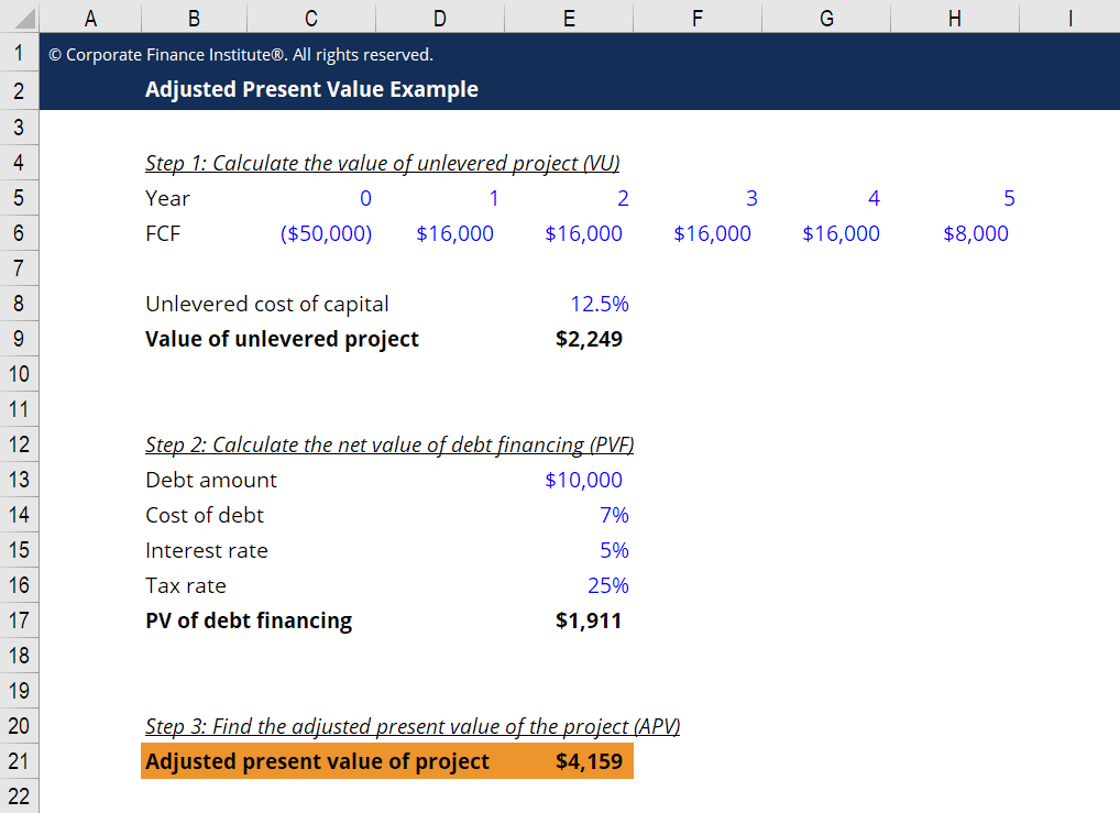
The APV method to calculate the levered value (VL) of a firm or project consists of three steps:

Step 1

Calculate the value of the unlevered firm or project (VU), i.e. its value with all-equity financing. To do this, discount the stream of FCFs by the unlevered cost of capital (rU).

Step 2

Calculate the net value of the debt financing (PVF), which is the sum of various effects, including:

•       PV(Interest tax shields) – our main focus
•       PV(Issuance costs)
•       PV(Financial distress costs)
•       PV(Other market imperfections)

Step 3

Sum up the value of the unlevered project and the net value of debt financing to find the adjusted present value of the project. That is, VL = VU + PVF.

Download the Free Template

Enter your name and email in the form below and download the free template now!

Applications of Adjusted Present Value

The APV method is most useful when evaluating companies or projects with a fixed debt schedule, as it can easily accommodate the side effects of financing such as interest tax shields. APV breaks down the value of a project into its fundamental components and thus provides useful information needed to refine the transaction and monitor its execution.

Leveraged buyouts (LBOs), where one firm acquires another firm using debt to finance the purchase, are a classical situation where APV is used. The APV method is the most practical for this situation because of the changing capital structure.

Other Metrics: WACC and FTE Methods

Weighted average cost of capital (WACC) is also a widely-accepted method of valuation and can be used in valuing levered firms. Comparably, it has a simpler structure.

A firm’s WACC is calculated as: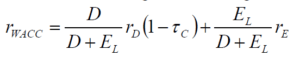 

Where D = the firm’s debt and E = firm’s equity, both at market values.

rD = cost of debt, rE = cost of equity, τ = tax rate.

The project value is computed by discounting streams of the firm’s free cash flow with WACC.

The Flow to Equity (FTE) method calculates the firm’s levered cash flow to equity (LCFE) using the following formula:

LCFE = Unlevered Cash Flow – Interest × (1 – tax rate),

LCFE is then discounted with rE to get the value of equity.

Total value is VL = E + D.

Both the WACC and FTE methods operate under the assumption that the firm will keep a fixed debt-to-equity ratio (D/E), implying that the firm will continue to raise debt at the same cost into the future. Realistically, however, this is often not the case. If D/E changes over time, WACC will also change, making the use of this method difficult. In general, if D/E remains constant over time, the WACC or FTE methods are easier to implement. However, the APV method is more practical when dealing with a complex debt schedule.

More Resources

Thank you for reading CFI’s guide to Adjusted Present Value (APV). To keep learning and mastering your corporate finance skills, we highly recommend these relevant articles:

• What is the WACC Formula?
• Leveraged Buyout
• Unlevered Beta
• Unlevered Cost of Capital
• See all valuation resources