RIGHT Function
Returns a specified number of characters from the end of a given text string
What is the RIGHT Function?
The RIGHT Function[1] is categorized under Excel TEXT functions. The function will return a specified number of characters from the end of a given text string.
In doing financial analysis, the RIGHT function can be useful if we wish to extract characters from the right side of a text string. Generally, it is used by combining it with other functions such as VALUE, SUM, COUNT, DATE, DAY, etc.
Formula
=RIGHT(text,[num_chars])
The RIGHT function uses the following arguments:
- Text (required argument) – This is the original text string.
- Num_chars (optional argument) – Specifies the number of characters to be returned from the end of the given text. It is the number of characters to be extracted starting on the right side of the text. If we omit the argument, the default value of 1 is taken.
How to Use the RIGHT Function in Excel
As a worksheet function, RIGHT can be entered as part of a formula in a cell of a worksheet. To understand the uses of the function, let us consider an example:
Example 1
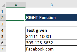
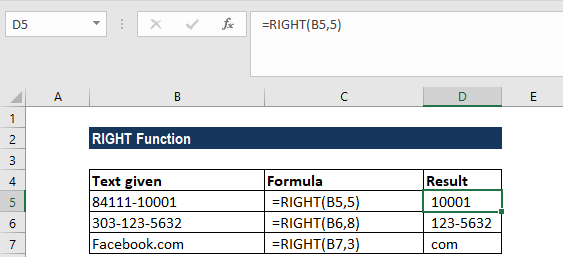
Suppose we wish to find certain characters from the data below:
The results in Excel are shown in the screenshot below:
Example 2
The RIGHT function always returns a text string, even though it contains digits and looks like a number. This is important if we wish to use the result of the function within other functions or formulas.
Using the VALUE function, we can ensure the number format is kept and the result is not converted to text.
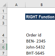
Let’s assume we wish to separate numbers from the data below:
We wish to extract the last 4 characters, the order number. The formula to use will be =VALUE(RIGHT(B5,4)), as shown below:
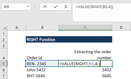
We get the results below:
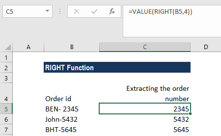
As we can see in the screenshot above, the numbers in column B obtained with a VALUE RIGHT formula are right-alighted in the cells, as opposed to left-aligned text in column A. Since Excel recognizes the output as numbers, we can sum or average the values, find the min and max value, or perform other calculations.
A Few Things To Remember About the RIGHT Function
- #VALUE! error – Occurs if the given [num_chars] argument is less than 0.
- Dates are stored in Excel as numbers, and it is only the cell formatting that makes them appear as dates in our spreadsheet. Hence, if we attempt to use the RIGHT function on a date, it will return the start characters of the number that represents that date.
For example, 01/01/1980 is represented by the number 29221, so applying the RIGHT function to a cell containing the date 01/01/1980 (and requesting that 4 characters be returned) will result in a returned value of “9221.” If we wish to use RIGHT on dates, we can combine it with the DAY, DATE, MONTH or YEAR functions. Otherwise, we can convert the cells containing dates to text using Excel’s Text to Columns tool.
Click here to download the sample Excel file
Connect what you just learned to a clear career path with CFI’s role‑based courses and certification programs.
Additional Resources
Thanks for reading CFI’s guide to important Excel functions! By taking the time to learn and master these functions, you’ll significantly speed up your financial analysis. To learn more, check out these additional CFI resources:
- Excel Functions for Finance
- Advanced Excel Formulas You Must Know
- Excel Shortcuts for PC and Mac
- ABSOLUTE Function in Excel
- LEFT Function
Article Sources
Excel Tutorial
To master the art of Excel, check out CFI’s Excel Crash Course, which teaches you how to become an Excel power user. Learn the most important formulas, functions, and shortcuts to become confident in your financial analysis.

Launch CFI’s Excel Crash Course now to take your career to the next level and move up the ladder!


