AVERAGEIF Function
Calculates the average of all numbers in a range of cells based on a given criterion
What is the AVERAGEIF Function?
The AVERAGEIF Function[1] is an Excel Statistical function, which calculates the average of a given range of cells by a specific criterion. Basically, AVERAGEIF calculates the central tendency, which is the location of the center of a group of numbers in a statistical distribution. The function was introduced in Excel 2007.
AVERAGEIF Formula
=AVERAGEIF(range, criteria, [average_range])
The AVERAGEIF function uses the following arguments:
- Range (required argument) – This is the range of one or more cells that we want to average. The argument may include numbers or names, arrays, or references that contain numbers.
- Criteria (required argument) – Criteria determines how the cell will be averaged. Criteria can be in the form of an expression, number, cell reference, or text that defines which cells are averaged. For example, 12, “<12”, “Baby” or C2.
- Average_range (optional argument) – This is the actual set of cells that we wish to average. If a user omits it, the function will use the range given.
How to Use the AVERAGEIF Function in Excel
This is a built-in function that can be used as a worksheet function in Excel. To understand the uses of the AVERAGEIF function, let’s consider a few examples:
Step-by-Step Example of AVERAGEIF
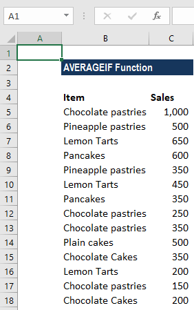
Generally, AVERAGEIF is commonly used in finding the average of cells that are an exact match of a given criterion. For example, from the table below, we wish to find out the sales of chocolate pastries. We are given the following data:
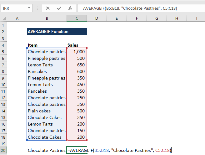
The formula used to find the average is below:
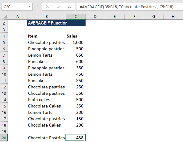
We get the result below:
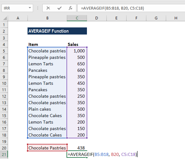
If we wish to avoid typing the condition in the formula, we can type in a separate cell and provide a reference to the cell in the formula, as shown below:
Example – How to Find the Average, with Wildcard Characters!
Let’s now see how we can use wildcards in the AVERAGEIF function. Using the data above, but now I wish to find out the average sales of all types of pastries sold.
As in our search, the keyword is to be preceded by some other character, so we will add an asterisk in front of the word. Similarly, we can use it at the end of the word if the keyword will be followed by some other character.
Now, the formula we will use would be =AVERAGEIF(B5:B18, “*Pastries”, C5:C18)
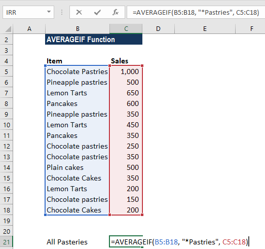
We will get the result below:
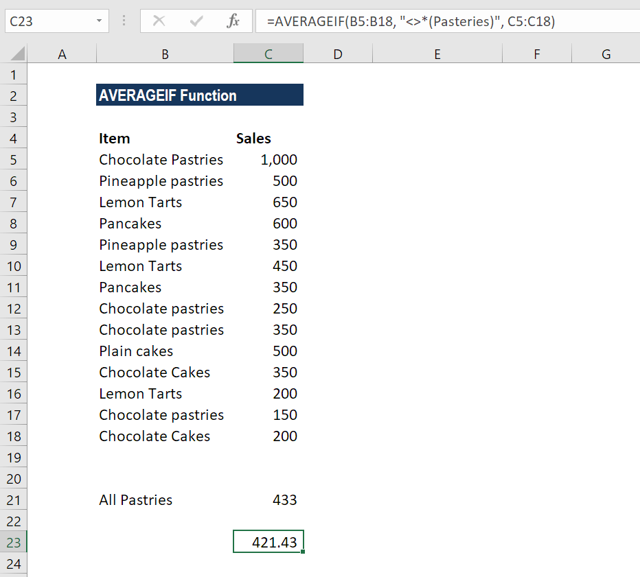
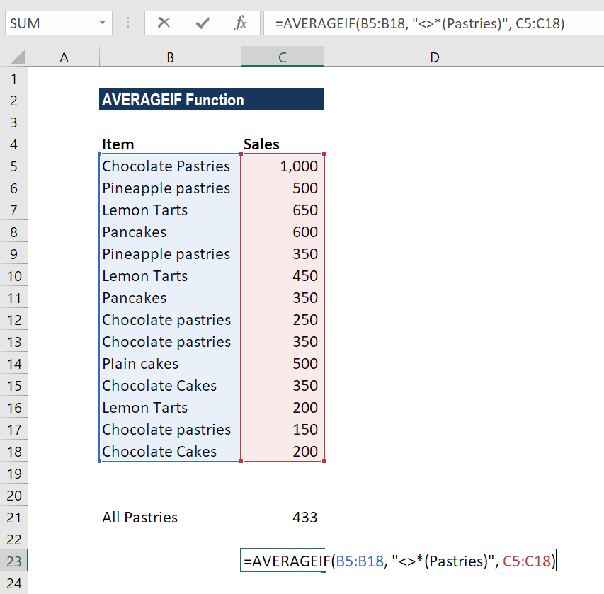
Suppose we wish to find out the average of all items except pastries, we will use the following formula =AVERAGEIF(A12:A15, “<>*(Pastries)”, B12:B15).
Example – How to Find an Average, with Empty or Not Empty Criteria
Sometimes, when doing data analysis in Excel, we may need to find an average of numbers that correspond to either empty or non-empty cells.
So, in order to include blank cells in the formula, we will enter “=” that is, the “equals” sign. The cell will not contain anything that is not a formula or zero-length string.
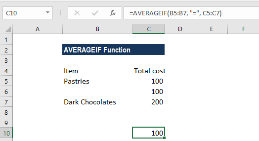
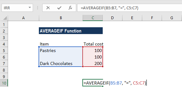
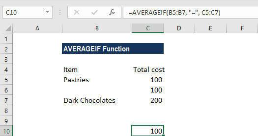
For example, we are given the total cost of preparation of three items. Using =AVERAGEIF(B5:B7, “=”, C5:C7) formula, Excel will calculate an average of cell B5:B7 only if a cell in Column A in the same row is empty, as shown below:
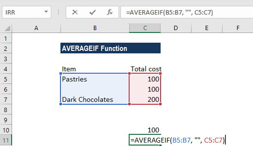
Suppose we wish to average values that correspond to blank cells and include empty strings that are returned by any other function. In such a scenario, we will use “” in the given criteria.
For example: =AVERAGEIF(B5:B7, “”, C5:C7)
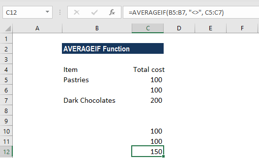
Now, suppose we wish to find the average of only those values that correspond to empty cells. In this scenario, we will use “<>” in the criteria.
So now using the same data, the formula to use is below:
The result will be the average of Pastries & Dark Chocolates, that is 150.
Things to Remember About the AVERAGEIF Function
- #DIV0! error – Occurs when:
- No cells in the range meet the criteria
- Range is a blank or text value
- When the given criteria is empty, AVERAGEIF treats it as 0 value.
- The use of wildcard characters such as the asterisk (*), the tilde(~) in the function as criteria, greatly enhances the search criteria. Example 2 shows a great way to use wildcard characters.
- The function will ignore cells that contain TRUE or FALSE.
Click here to download the sample Excel file
Connect what you just learned to a clear career path with CFI’s role‑based courses and certification programs.
Additional Resources
Thanks for reading CFI’s guide to important Excel functions! By taking the time to learn and master these functions, you’ll significantly speed up your financial analysis. To learn more, check out these additional CFI resources:
- Excel Functions for Finance
- Advanced Excel Formulas Course
- Advanced Excel Formulas You Must Know
- Excel Shortcuts for PC and Mac
Article Sources
Excel Tutorial
To master the art of Excel, check out CFI’s Excel Crash Course, which teaches you how to become an Excel power user. Learn the most important formulas, functions, and shortcuts to become confident in your financial analysis.

Launch CFI’s Excel Crash Course now to take your career to the next level and move up the ladder!


