COLUMN Function in Excel
Returns the column number of a given cell reference
What is the COLUMN Function in Excel?
The COLUMN Function[1] in Excel is a Lookup/Reference function. This function is useful for looking up and providing the column number of a given cell reference. For example, the formula =COLUMN(A10) returns 1, because column A is the first column.
Formula
=COLUMN([reference])
The COLUMN function uses only one argument – reference – which is an optional argument. It is the cell or a range of cells for which we want the column number. The function will give us a numerical value.
A few points to remember for the reference argument:
- Reference can be a single cell address or a range of cells.
- If not provided by us, then it will default to the cell in which the column function exists.
- We cannot include multiple references or addresses as reference for this function
How to use the COLUMN Function in Excel?
It is a built-in function that can be used as a worksheet function in Excel. To understand the uses of the COLUMN Function in Excel, let’s consider a few examples:
Example 1
Suppose we are given the following references:
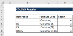
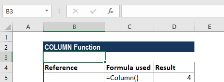
In the first reference that we’ve provided, we did not give a reference so it gave us the result 4 with the COLUMN function in cell C5, as shown in the screenshot below:
When we used the reference B6, it returned the result of 3 as the column reference was B.
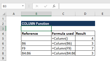
As you can see above, when we provide an array, the formula returned a result of 3.
Example 2
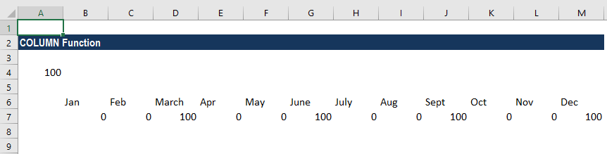
Suppose a flower expense is payable every third month. The flower expense is $100. If we wish to generate a fixed value every third month, we can use a formula based on the MOD function.
The formula used is =IF(MOD(COLUMN(B8)-1,3)=0,$A$2,0), as shown below:
So, in the example above, we took a recurring expense at every 3 months. If we wish to get it once in 2 months, then we will change the formula to:
=IF(MOD(COLUMN(B19)-1,2)=0,$A$4,0)
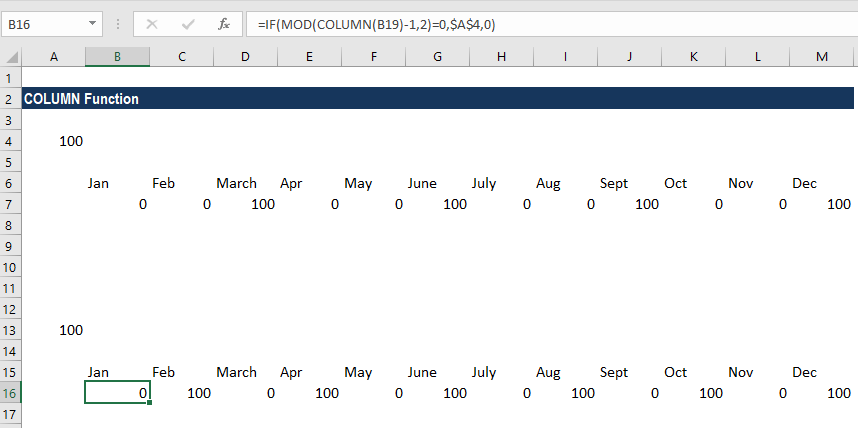
The formula can also be used for a fixed expense every regular time interval, a fixed payment every 6 months such as premiums, etc.
Here, two formulas are used: MOD and COLUMN. MOD is the main function used. The function is useful for formulas that are required to do a specified act every nth time. Here, in our example, the number was created with the COLUMN function, which returned the column number of cell B8, the number 2, minus 1, which is supplied as an “offset.” Why did we use an offset? It is because we wanted to make sure that Excel starts counting at 1, regardless of the actual column number.
The divisor is fixed as 3 (flower expense) or 2, since we want to do something every 3rd or 2nd month. By testing for a zero remainder, the expression will return TRUE at the 3rd , 6th , 9th , and 12th months or at the 2nd, 4th, 6th, 8th, 10th and 12th months.
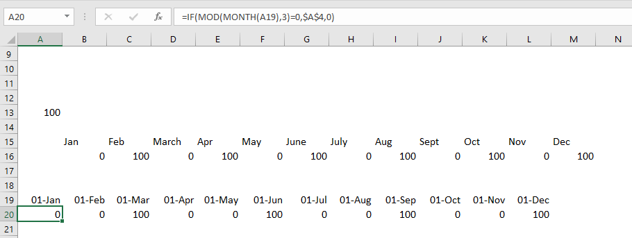
Using the formula and working with a date
As shown in the screenshot below, we can use a date instead of using a text value as we’ve used for months. This will help us in building a more rational formula. All we need to do is adjust the formula to extract the month number and use that instead of the column number:
=IF(MOD(MONTH(A19),3)=0,$A$4,0)
Example 3
If we want, we can use this column function to get the sum of every nth column. Suppose we are given the following data:
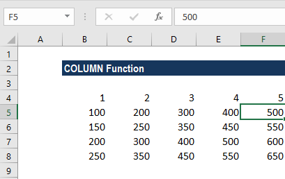
As we wish to sum every nth column, we used a formula combing three Excel functions: SUMPRODUCT, MOD, and COLUMN.
The formula used is:
=SUMPRODUCT(–(MOD(COLUMN(B4:F4)-COLUMN(B4)+1,G4)=0),B4:F4)
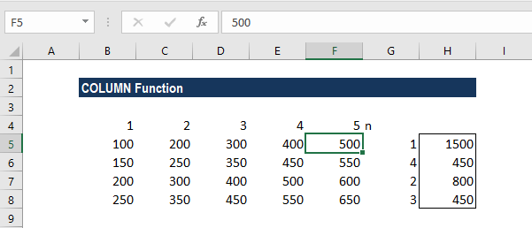
Let us see how the COLUMN Function in Excel works.
In the formula above, Column G is the value of n in each row. Using the MOD function will return the remainder for each column number after dividing it by N. So, for example, when N = 3, MOD will return something like this:
{1,2,0,1,2,0,1,2,0}
So, the formula uses =0 to get TRUE when the remainder is zero and FALSE when it is not. Note that we used a double-negative (–) to get TRUE or FALSE to ones and zeros. It gives an array like this:
{0,0,1,0,0,1,0,0,1}
Where 1s now indicate “nth values.” It goes into SUMPRODUCT as array1, along with B5:F5 as array2. Now SUMPRODUCT multiplies and then adds the products of the arrays.
So, the only values of that last multiplication are those where array1 contains 1. In this way, we can think of the logic of array1 “filtering” the values in array2.
Click here to download the sample Excel file
Additional Resources
Thanks for reading CFI’s guide to important Excel functions! By taking the time to learn and master these functions, you’ll significantly speed up your financial analysis. To learn more, check out these additional CFI resources:
- Excel Functions for Finance
- Advanced Excel Formulas Course
- Advanced Excel Formulas You Must Know
- Excel Shortcuts for PC and Mac
- See all Excel resources
Article Sources
Excel Tutorial
To master the art of Excel, check out CFI’s Excel Crash Course, which teaches you how to become an Excel power user. Learn the most important formulas, functions, and shortcuts to become confident in your financial analysis.

Launch CFI’s Excel Crash Course now to take your career to the next level and move up the ladder!


