CONCATENATE Function

What is the CONCATENATE Function?

The CONCATENATE Function[1] is categorized under Excel Text Functions. The function helps to join two or more strings into one string.

As a financial analyst, we often deal with data when doing financial analysis. The data is not always structured for analysis and we often need to combine data from one or more cells into one cell or split data from one cell into different cells. The CONCATENATE function helps us to do that.

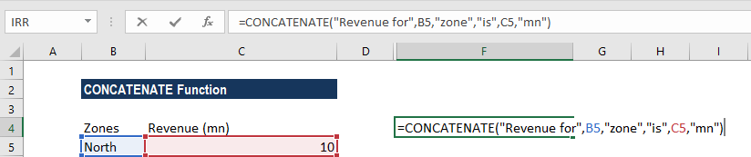
For example, If I get a list of projects in this format:

The CONCATENATE function helps structure data in the following format:

Formula

=CONCATENATE(text1, [text2], …)

The CONCATENATE function uses the following arguments:

1. Text1 (required argument) – This is the first item to join. The item can be a text value, cell reference, or a number.
2. Text2 (required argument) – The additional text items that we wish to join. We can join up to 255 items that are up to 8192 characters.

How to use the CONCATENATE Function in Excel?

To understand the uses of this function, let’s consider a few examples:

Example 1

Suppose you wish to make your data easy to comprehend for users. This function helps to do that.

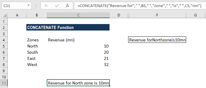
Using the monthly sales data below:

We can use the formula:

To get the following result:

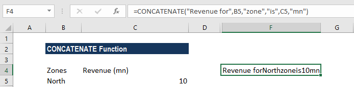
This result is unacceptable as it is difficult to read. For this, we need to add spaces. We would add a space (” “) in between the combined values so that the result displays “Revenue for North zone is 10mn.” The formula to use is:

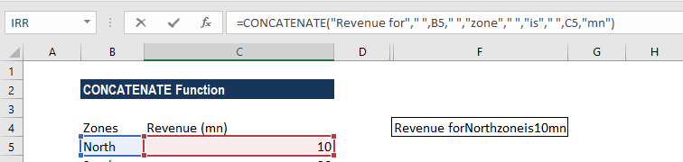
We get the following result:

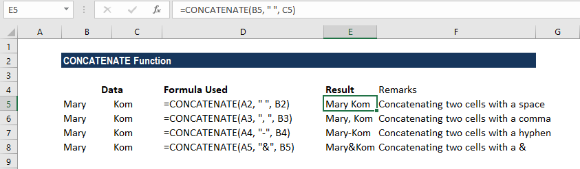
Example 2

While analyzing and presenting data, we may often need to join values in a way that includes commas, spaces, various punctuation marks, or other characters such as a hyphen or slash. To do this, all we need to do is include the character we want in our concatenation formula, but we need to enclose that character in quotation marks. A few examples are shown below:

Example 3

Sometimes our data needs to be separated by a line break instead of spaces or a character as shown in the previous examples. The most common example is merging mailing addresses imported from a .csv file or PDF file.

While doing so, we cannot simply type a line break in the formula like a regular character, and therefore a special CHAR function is needed to supply the corresponding ASCII code to the concatenation formula.

Hence, in Windows, we use CHAR(10) where 10 is the ASCII code for line feed. On the Mac system, we use CHAR(13) where 13 is the ASCII code for a carriage return.

In the screenshot below, we place the address information in columns A through D, and we are putting them together in column E by using the concatenation operator “&”. The merged values are separated with a comma (“, “), space (” “) and a line break CHAR(10):

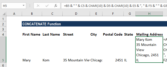
The formula used was:

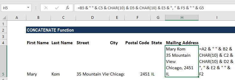
To get the result, as shown above, we need to enable the “Wrap text” option for the results to display properly. To do this, use Ctrl + 1 to open the Format Cells dialog. Switch to the Alignment tab and check the Wrap text box or go to Home tab and under Alignment click on Wrap text.

Example 4

When combining values from multiple cells, we must make some effort, as this function does not accept arrays and requires a single cell reference in each argument.

So we need to use formula =CONCATENATE(B1, B2, B3, B4) or =B1 & B2 & B3 & B4.

Let’s see how to do this quickly using the TRANSPOSE function. Suppose there are 78 cells that need to be concatenated. In such a scenario, we need to:

• Select the cell where we want to output the concatenated range. D1 in our example.
• Then enter the TRANSPOSE formula in that cell, =TRANSPOSE(A1:A78).
• Now in the formula bar, press F9 to replace the formula with calculated values.
• Delete the curly braces as shown below:

• Now type =CONCATENATE in front of the cell references in the Formula bar, put an open parenthesis and closing parenthesis, and then press Enter.

The result would be:

A few notes about the CONCATENATE Function

1. The CONCATENATE function will give the result as a text string.
2. The function converts numbers to text when they are joined.
3. The function doesn’t recognize arrays. Hence, we need to provide each cell reference separately.
4. #VALUE! error – Occurs when at least one of the CONCATENATE function’s arguments is invalid.
5. Numbers don’t need to be in quotation marks.
6. #NAME? error – Occurs when there are quotation marks missing from a Text argument.
7. The ampersand (&) calculation operator lets us join text items without using a function. For example, =A1 & B1 will return the same value as =CONCATENATE(A1,B1). In many cases, using the ampersand operator is quicker and simpler than using CONCATENATE to create strings.

Click here to download the sample Excel file

Additional Resources

Thanks for reading CFI’s guide to important Excel functions! By taking the time to learn and master these functions, you’ll significantly speed up your financial analysis. To learn more, check out these additional CFI resources:

• Advanced Excel Formulas Course
• CONCAT Function
• CLEAN Function
• QUARTILE Function
• See all Excel resources