INDEX Function
Get the value at a given position in a range or array
What is the INDEX Function?
The INDEX Function[1] is categorized under Excel Lookup and Reference functions. The function will return the value at a given position in a range or array. The INDEX function is often used with the MATCH function. We can say it is an alternative way to do VLOOKUP.
As a financial analyst, INDEX can be used in other forms of analysis besides looking up a value in a list or table. In financial analysis, we can use it along with other functions, for lookup and to return the sum of a column.
There are two formats for the INDEX function:
- Array format
- Reference format
The Array Format of the INDEX Function
The array format is used when we wish to return the value of a specified cell or array of cells.
Formula
=INDEX(array, row_num, [col_num])
The function uses the following arguments:
- Array (required argument) – This is the specified array or range of cells.
- Row_num (required argument) – Denotes the row number of the specified array. When the argument is set to zero or blank, it will default to all rows in the array provided.
- Col_num (optional argument) – This denotes the column number of the specified array. When this argument is set to zero or blank, it will default to all rows in the array provided.
The Reference Format of the INDEX Function
The reference format is used when we wish to return the reference of the cell at the intersection of row_num and col_num.
Formula
=INDEX(reference, row_num, [column_num], [area_num])
The function uses the following arguments:
- Reference (required argument) – This is a reference to one or more cells. If we input multiple areas directly into the function, individual areas should be separated by commas and surrounded by brackets. Such as (A1:B2, C3:D4), etc.
- Row_num (required argument) – Denotes the row number of a specified area. When the argument is set to zero or blank, it will default to all rows in the array provided.
- Col_num (optional argument) – This denotes the column number of the specified array. When the argument is set to zero or blank, it will default to all rows in the array provided.
- Area_num (optional argument) – If the reference is supplied as multiple ranges, area_num indicates which range to use. Areas are numbered by the order they are specified.
If the area_num argument is omitted, it defaults to the value 1 (i.e., the reference is taken from the first area in the supplied range).
How to Use the INDEX Function in Excel
To understand the uses of the function, let us consider a few examples:
Example 1
We are given the following data and we wish to match the location of a value.
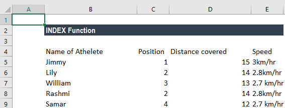
In the table above, we wish to see the distance covered by William. The formula to use will be:
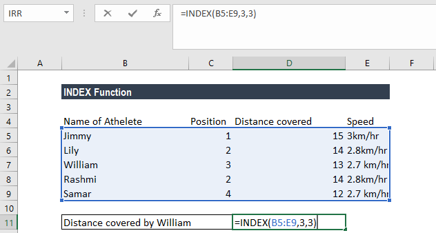
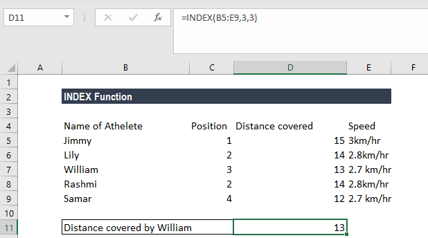
We get the result below:
Example 2
Now let’s see how to use the MATCH and INDEX functions at the same time. Suppose we are given the following data:
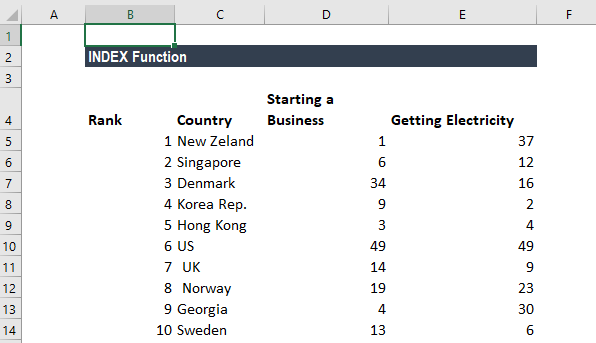
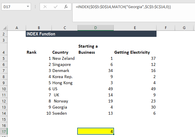
Suppose we wish to find out Georgia’s rank in the Ease of Doing Business category. We will use the following formula:
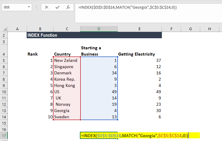
Here, the MATCH function will look up for Georgia and return number 10 as Georgia is 10 on the list. The INDEX function takes “10” in the second parameter (row_num), which indicates which row we wish to return a value from and turns into a simple =INDEX($C$2:$C$11,3).
We get the result below:
What is INDEX MATCH in Excel?
The INDEX MATCH Formula is the combination of two functions in Excel: INDEX and MATCH.
=INDEX() returns the value of a cell in a table based on the column and row number.
=MATCH() returns the position of a cell in a row or column.
Combined, the two formulas can look up and return the value of a cell in a table based on vertical and horizontal criteria. For short, this is referred to as just the Index Match function. To see a video tutorial, check out our free Excel Crash Course.
How to Use the MATCH Formula
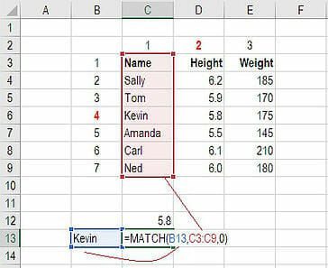
Sticking with the same example as above, let’s use MATCH to figure out what row Kevin is in.
Follow the steps below:
- Type “=MATCH(” and link to the cell containing “Kevin”… the name we want to look up.
- Select all the cells in the Name column (including the “Name” header).
- Type zero “0” for an exact match.
- The result is that Kevin is in row “4.”
![]()
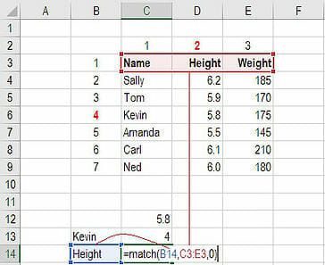
Use MATCH again to figure out what column Height is in.
Follow the steps below:
- Type “=MATCH(” and link to the cell containing “Height”… the criteria we want to look up.
- Select all the cells across the top row of the table.
- Type zero “0” for an exact match.
- The result is that Height is in column “2.”
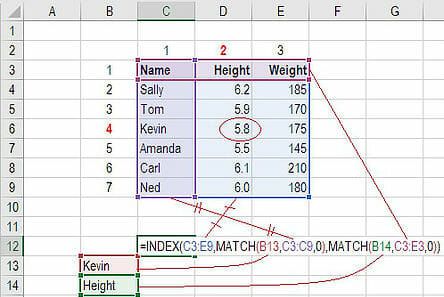
How to Combine INDEX and MATCH
Now, we can take the two MATCH formulas and use them to replace the “4” and the “2” in the original INDEX formula. The result is an INDEX MATCH formula.
Follow the steps below:
- Cut the MATCH formula for Kevin and replace the “4” with it.
- Cut the MATCH formula for Height and replace the “2” with it.
- The result is Kevin’s Height is “5.8.”
- Congratulations, you now have a dynamic INDEX MATCH formula!
Video Explanation of How to Use Index Match in Excel
Below is a short video tutorial on how to combine the two functions and effectively use Index Match in Excel! Check out more free Excel tutorials on CFI’s YouTube Channel.
Hopefully, the short video above makes it even clearer how to use the two functions to dramatically improve your lookup capabilities in Excel.
Things to Remember About the INDEX Function
- #VALUE! error – Occurs when any of the given row_num, col_num or area_num arguments are non-numeric.
- #REF! error – Occurs due to either of the following reasons:
- The given row_num argument is greater than the number of rows in the given range;
- The given [col_num] argument is greater than the number of columns in the range provided; or
- The given [area_num] argument is more than the number of areas in the supplied range.
- VLOOKUP vs. INDEX function
- Excel VLOOKUP is unable to look to its left, meaning that our lookup value should always reside in the left-most column of the lookup range. This is not the case with the INDEX and MATCH functions.
- VLOOKUP formulas get broken or return incorrect results when a new column is deleted from or added to a lookup table. With INDEX and MATCH, we can delete or insert new columns in a lookup table without distorting the results.
Click here to download the sample Excel file
Connect what you just learned to a clear career path with CFI’s role‑based courses and certification programs.
Additional Resources
Thank you for reading CFI’s guide to the INDEX Function. To learn more, check out these additional CFI resources:
- Advanced Excel Formulas Course
- Advanced Excel Formulas You Must Know
- Excel Shortcuts for PC and Mac
- Financial Analyst Program
- Best Excel Courses for Finance
Article Sources
Excel Tutorial
To master the art of Excel, check out CFI’s Excel Crash Course, which teaches you how to become an Excel power user. Learn the most important formulas, functions, and shortcuts to become confident in your financial analysis.

Launch CFI’s Excel Crash Course now to take your career to the next level and move up the ladder!


