GETPIVOTDATA Function
Extracts data from specified fields in an Excel Pivot Table
What is the GETPIVOTDATA Function?
The GETPIVOTDATA Function[1] is categorized under Excel Lookup and Reference functions. The function helps to extract data from specified fields in an Excel Pivot Table.
The Pivot Table is used often in financial analysis to facilitate deeper analysis of given data. The function helps extract, group, or add data from a pivot table.
Formula
=GETPIVOTDATA(data_field, pivot_table, [field1, item1, field2, item2], …)
The GETPIVOTDATA function uses the following arguments:
- Data_field (required argument) – This is the worksheet information from which we intend to remove nonprintable characters.
- Pivot_table (required argument) – This is a reference to a cell, range of cells, or named range of cells in a pivot table. We use the reference to specify the pivot table.
- Field1, Item1, Field2, Item2 (optional argument) – This is a field/item pair. There are up to 126 pairs of field names and item names that may be used to describe the data that we wish to retrieve.
We need to enclose in quotation marks all field names and names for items other than dates and numbers. We need to keep in mind the following:
- Dates are entered as date serial numbers by using the DATE function so that they are in the proper date format.
- Numbers can be entered directly.
- Time should be entered in decimals or as the TIME function.
How to Use GETPIVOTDATA Function in Excel
To understand the uses of the GETPIVOTDATA function, let’s consider a few examples:
Example 1
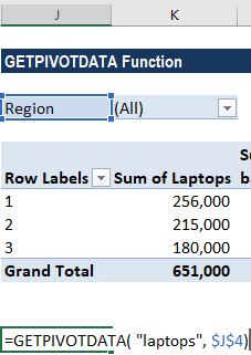
Let’s assume we are given the pivot table below:
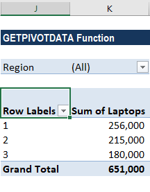
Suppose we wish to get the sum of laptops from the pivot table given above. In such a scenario, we will use the formula =GETPIVOTDATA( “laptops”, $J$4) and get the result as 651,000.
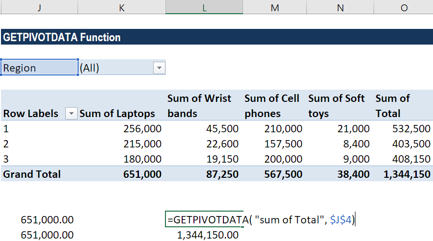
Continuing with the same example, suppose we are given the pivot table below:
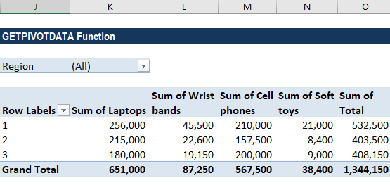
Now we wish to get the total sales. The formula to use will be =GETPIVOTDATA( “sum of Total”, $J$4).
Example 2
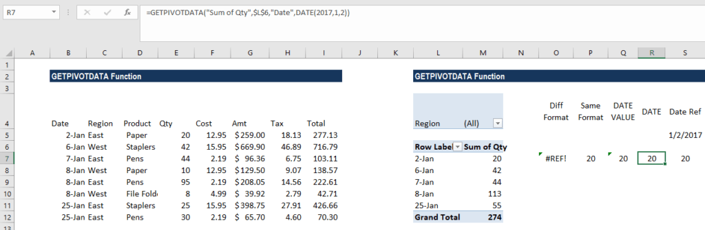
Using dates in the GETPIVOTDATA function may sometimes produce an error. Suppose we are given the following data:
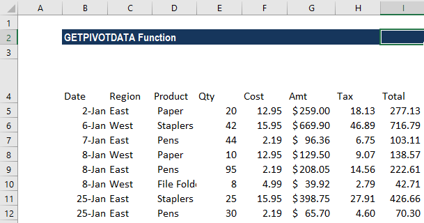
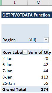
We drew the following pivot table from it:
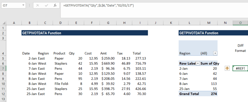
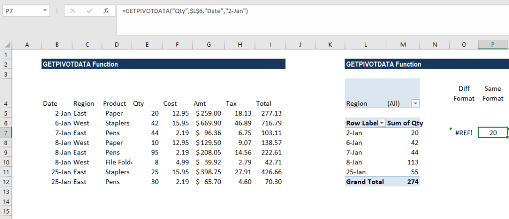
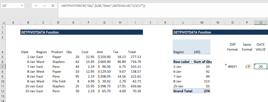
If we use the formula =GETPIVOTDATA(“Qty”,$L$6,”Date”,”1/2/17″), we will get a REF! error:
To prevent such date errors, we can use any of the following methods:
- Match the Pivot Table’s date format – In order to get the correct, error-free results, we will use the same date format as in the pivot table. For example, we took 2-Jan as shown below:
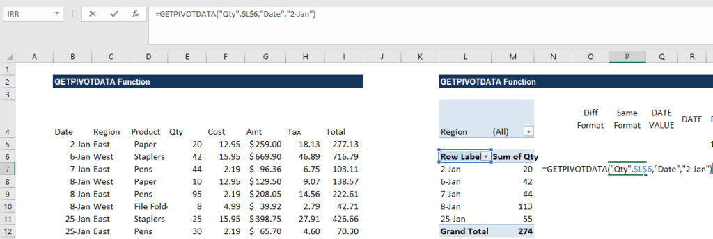
As seen below, the same format gives us the desired result:
- Use the GETPIVOTDATA function with the DATEVALUE function – Here, instead of just typing the date in the formula, add the DATEVALUE function to the date. As shown below, the formula will be:
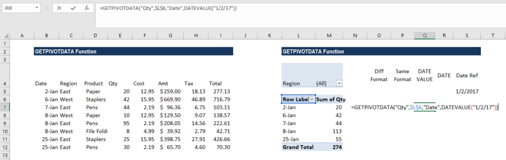
We will get the result below:
- Use the GETPIVOTDATA function with the DATE function – Here, instead of just typing the date in the formula, we will add the DATE function. As shown below, the formula will be:
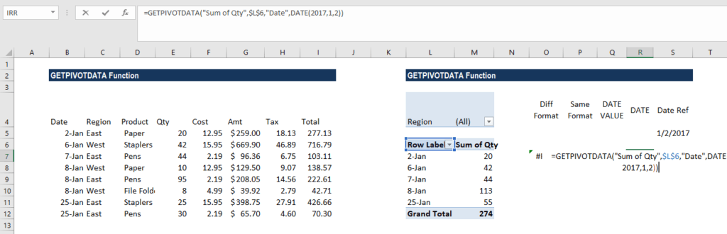
We will get the result below:
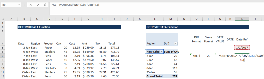
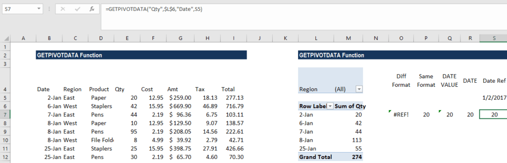
- Use the GETPIVOTDATA function with the DATE Function – Example 2: Here, instead of just typing the date in the formula, we can refer to a cell that contains a valid date, in any format recognized as a date by MS Excel. The formula to be used is =GETPIVOTDATA(“Qty”,$L$6,”Date”,S5).
We will get the result below:
A Few Notes About the GETPIVOTDATA Function
- #REF! error – Occurs when:
- The given pivot_table reference does not relate to a pivot table.
- When we provide invalid fields for the arguments data_field, [field], or [item].
- The field details are not displayed in the specified pivot table.
- Remember that if an item contains a date, it should be in date format or serial number.
- The function can be automatically inserted by enabling the “Use GetPivotData functions for PivotTable references” option in MS Excel.
Click here to download the sample Excel file
Connect what you just learned to a clear career path with CFI’s role‑based courses and certification programs.
Additional Resources
Thanks for reading CFI’s guide to important Excel functions! By taking the time to learn and master these functions, you’ll significantly speed up your financial analysis. To learn more, check out these additional CFI resources:
- Excel Functions for Finance
- Advanced Excel Formulas Course
- Advanced Excel Formulas You Must Know
- Excel Shortcuts for PC and Mac
Article Sources
Excel Tutorial
To master the art of Excel, check out CFI’s Excel Crash Course, which teaches you how to become an Excel power user. Learn the most important formulas, functions, and shortcuts to become confident in your financial analysis.

Launch CFI’s Excel Crash Course now to take your career to the next level and move up the ladder!


