
Get In-Demand Finance Certifications
Looks up value in a row
HLOOKUP stands for Horizontal Lookup and can be used to retrieve information from a table by searching a row for the matching data and outputting from the corresponding column. While VLOOKUP searches for the value in a column, HLOOKUP searches for the value in a row.
=HLOOKUP(value to look up, table area, row number)
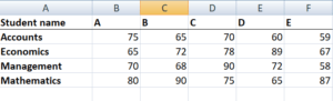
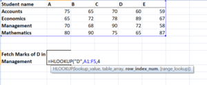
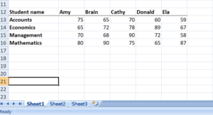
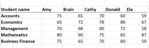
Let us consider the example below. The marks of four subjects for five students are as follows:
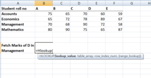
Now, if our objective is to fetch the marks of student D in Management, we can use HLOOKUP as follows:
The HLOOKUP function in Excel comes with the following arguments:
HLOOKUP(lookup_value, table_array, row_index_num, [range_lookup])
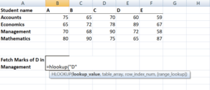
As you can see in the screenshot above, we need to give the lookup_value first. Here, it would be student D as we need to find his marks in Management. Now, remember that lookup_value can be a cell reference or a text string, or it can be a numerical value as well. In our example, it would be student name as shown below:
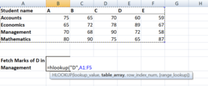
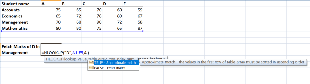
The next step would be to give the table array. Table array is nothing but rows of data in which the lookup value would be searched. Table array can be a regular range or a named range, or even an Excel table. Here, we will give row A1:F5 as the reference.
Next, we would define ‘row_index_num,’ which is the row number in the table_array from where the value would be returned. In this case, it would be 4, as we are fetching the value from the fourth row of the given table.
Suppose, if we require marks in Economics, then we would put row_index_num as 3.
The next is range_lookup. It makes HLOOKUP search for exact or approximate value. As we are looking out for an exact value, it would be False.
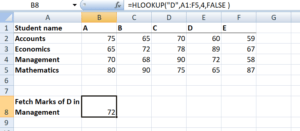
The result would be 72.
Here, HLOOKUP is searching for a particular value in the table and returning an exact or approximate value.
Let’s understand this using an example.
Suppose we are given names of student and marks below:
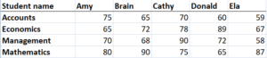
If we need to use the Horizontal Lookup formula to find the Math marks of a student whose name starts with a ‘D,’ the formula will be:

The wild character used is ‘*’.
4. #N/A error – It would be returned by HLOOKUP if ‘range_lookup’ is FALSE and the HLOOKUP function is unable to find the ‘lookup_value’ in the given range. We can embed the function in IFERROR and display our own message, for example: =IFERROR(HLOOKUP(A4, A1:I2, 2, FALSE), “No value found”).
5. If the ‘row_index_num’ < 1, HLOOKUP would return #VALUE! error. If ‘row_index_num’ > number of columns in ‘table_array’, then it would give #REF! error.
6. Remember HLOOKUP function in Excel can return only one value. This would be the first value n that matches the lookup value. What if there are a few identical records in the table? In that scenario, it is advisable to remove them or create a Pivot table and group them. The array formula can then be used on the Pivot table to extract all duplicate values that are present in the lookup range.
To learn more, launch our free Excel crash course now!
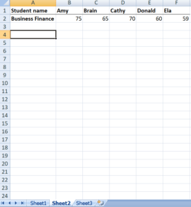
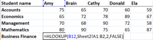
It means giving an external reference to our HLOOKUP formula. Using the same table, the marks of students in subject Business Finance are given in sheet 2 as follows:
We will use the following formula:
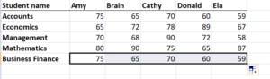
Then we will drag it to the remaining cells.
So far, we’ve used HLOOKUP for a single value. Now, let’s use it to obtain multiple values.
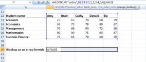
As shown in the table above, if I need to extract the marks of Cathy in all subjects, then I need to use the following formula:
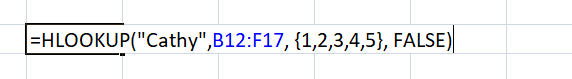
If you wish to get an array, you need to select the number of cells that are equal to the number of rows that you want HLOOKUP to return.
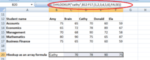
After typing FALSE, we need to press Ctrl + Shift + Enter instead of the Enter key. Why do we need to do so?
Ctrl + Shift + Enter will enclose the HLOOKUP formula in curly brackets. As shown below, all cells will give the results in one go. We will be saved from having to type the formula in each cell.
Connect what you just learned to a clear career path with CFI’s role‑based courses and certification programs.
Thank you for reading CFI’s guide on the HLOOKUP Function. To keep learning and advancing your career, the following resources will be helpful:
To master the art of Excel, check out CFI’s Excel Crash Course, which teaches you how to become an Excel power user. Learn the most important formulas, functions, and shortcuts to become confident in your financial analysis.

Launch CFI’s Excel Crash Course now to take your career to the next level and move up the ladder!


