IPMT Function

What is the IPMT Function?

The IPMT Function[1] is categorized under Excel Financial functions. The function calculates the interest portion based on a given loan payment and payment period. We can calculate, using IPMT, the interest amount of a payment for the first period, last period, or any period in between.

As a financial analyst, we will often be interested in knowing the principal component and interest component of a loan payment for a specific period. IPMT helps to calculate the amount.

Formula

=IPMT(rate, per, nper, pv, [fv], [type])

The IPMT function uses the following arguments:

1. Rate (required argument) – This is the interest per period.
2. Per (required argument) – This is the period for which we want to find the interest and must be in the range from 1 to nper.
3. Nper (required argument) – The total number of payment periods.
4. Pv (required argument) – This is the present value, or the lump sum amount, that a series of future payments is worth as of now.
5. Fv (optional argument) – The future value or a cash balance that we wish to attain after the last payment is made. If we omit the Fv argument, the function assumes it to be zero. The future value of a loan would be taken as zero.
6. Type (optional argument) – Accepts the numbers 0 or 1 and indicates when payments are due. If omitted, it is assumed to be 0. Set type to 0 if payments are at the end of the period, and to 1 if payments are due at the start.

How to use the IPMT Function in Excel?

As a worksheet function, IPMT can be entered as part of a formula in a cell of a worksheet.

To understand the uses of the IPMT function, let us consider a few examples:

Example 1

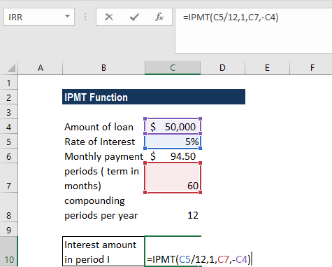
Let us assume we are given the following data:

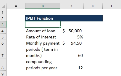
We will use the IPMT function to calculate the interest payments during months 1 and 2 of a $50,000 loan, which is to be paid off in full after 5 years. Interest is charged at a rate of 5% per year and the payment of the loan is to be made at the end of each month.

The formula to be used will be =IPMT( 5%/12, 1, 60, 50000).

The results are shown below:

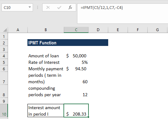
In the example above:

• As the payments are made monthly, it was necessary to convert the annual interest rate of 5% into a monthly rate (=5%/12), and the number of periods from years to months (=5*12).
• With the forecast value = 0 and the payment to be made at the end of the month, the [fv] and [type] arguments can be omitted from the above functions.
• The returned interest payments are negative values, as these represent outgoing payments (for a business taking out a loan) – that is why we took the loan amount as negative (-B2).

Things to remember about the IPMT function

1. We need to ensure that the units we use for specifying the rate and nper arguments are proper. If we make monthly payments on a 4-year loan at 24% annual interest, we need to use 24%/12 for rate and 4*24 for nper. If you make annual payments on the same loan, use 24% for rate and 4 for nper.
2. Cash paid out (as on a loan) is shown as negative numbers. Cash received (as from an investment) is shown as positive numbers.
3. #NUM! error – Occurs if the supplied per argument is less than zero or is greater than the supplied value of nper.
4. #VALUE! error – Occurs when any of the given arguments are non-numeric.

Click here to download the sample Excel file

Additional Resources

Thanks for reading CFI’s guide to important Excel functions! By taking the time to learn and master these functions, you’ll significantly speed up your financial analysis. To learn more, check out these additional CFI resources:

• Excel Functions for Finance
• Advanced Excel Formulas Course
• Advanced Excel Formulas You Must Know
• Excel Shortcuts for PC and Mac
• See all Excel resources