ISEVEN Function
Returns TRUE if the number is even or FALSE if the number is not even (or odd)
What is the ISEVEN Function?
The ISEVEN Function[1] is categorized under Excel Information functions. ISEVEN will return TRUE if the number is even or FALSE if the number is not even, or odd.
In financial analysis, we need to deal with numbers. The ISEVEN function is useful in data analysis where we need to understand the evenness and oddness of numbers.
Formula
=ISEVEN(number)
The ISEVEN function uses the following argument:
- Number (required argument) – This is the value we wish to test. If it is not an integer, the value is truncated.
How to use the ISEVEN Function in Excel?
To understand the uses of the ISEVEN function, let’s consider a few examples:
Example 1
Let’s see the results from the function when we provide the following data:
| Data | Formula | Result | Remarks |
|---|---|---|---|
| 210 | =ISEVEN(210) | TRUE | It tests if the number is even or not and returns TRUE or FALSE. |
| 2.9 | =ISEVEN(2.9) | TRUE | It truncates the decimal portion, which is 0.9. |
| 0 | =ISEVEN(0) | TRUE | Zero is considered even. Remember that the function evaluates empty cells to zero and returns TRUE if supplied with a reference to an empty cell. |
| 25 | =ISEVEN(25) | FALSE | Tests whether 25 is even or odd. |
| 08/22/2016 | =ISEVEN(08/22/2016) | TRUE | It tests the date here. The function tests the decimal representation of 08/22/2016, which is 42604. |
| 24/4 | =ISEVEN(24/4) | TRUE | Calculates if the result is even or odd when 24 is divided by 4 |
Example 2
Suppose we are given the following data:
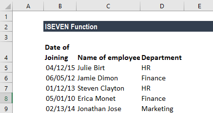
If we wish to highlight all even rows in the table above, we can use conditional formatting. The formula to use here will be ISEVEN. For example, as we wish to highlight the even rows, we will first select the entire range of data and then create conditional formatting rules that will use the formula =ISEVEN(ROW(B4:D9)).
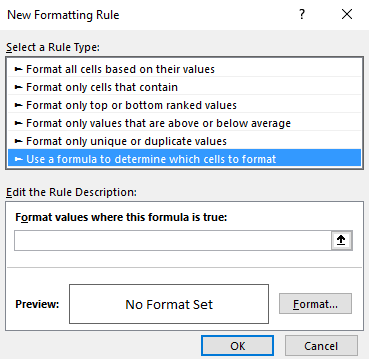
How to create conditional formatting:
Under Home tab – Styles, click on Conditional formatting. Click on New rule and then select – Use a formula to determine which cells to format:
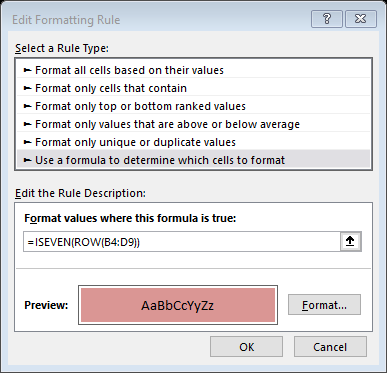
Enter the formula as shown below:
We get the results below:
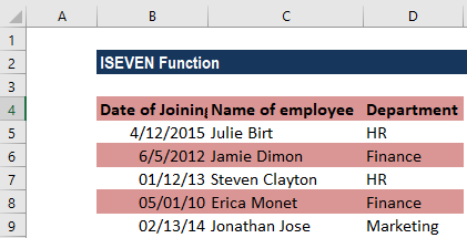
How the formula worked:
When we use a formula to apply conditional formatting, the formula will evaluate every cell in the selected range. As there are no addresses in the formula, for every cell in the data, the ROW and ISEVEN functions are run. ROW will return the row number of the cell, and ISEVEN returns TRUE if the row number is even and FALSE if the row number is odd. The rule will trigger TRUE, so even rows will be shaded as specified by us.
IF we wish to color odd rows, we can use ISODD function in such a scenario.
Things to remember about the ISEVEN Function
- #VALUE! error – Occurs when the given argument is non-numeric.
- We can insert a reference to a cell as seen in the above examples or the number directly in double quotes to get the desired result.
- The function was introduced in MS Excel 2007 and hence unavailable in earlier versions. It will return an error if we use it in older versions. For earlier versions, we can use the MOD function.
- ISEVEN is the opposite of the ISODD function.
Click here to download the sample Excel file
Additional Resources
Thanks for reading CFI’s guide to important Excel functions! By taking the time to learn and master these functions, you’ll significantly speed up your financial analysis. To learn more, check out these additional CFI resources:
- Excel Functions for Finance
- Advanced Excel Formulas You Must Know
- Excel Shortcuts for PC and Mac
- ISODD Function
- See all Excel resources
Article Sources
Excel Tutorial
To master the art of Excel, check out CFI’s Excel Crash Course, which teaches you how to become an Excel power user. Learn the most important formulas, functions, and shortcuts to become confident in your financial analysis.

Launch CFI’s Excel Crash Course now to take your career to the next level and move up the ladder!


