MATCH Function
Get the position of a value within an array
What is the MATCH Function?
The MATCH Function[1] is categorized under Excel Lookup and Reference functions. It looks up a value in an array and returns the position of the value within the array. For example, if we wish to match the value 5 in the range A1:A4, which contains values 1,5,3,8, the function will return 2, as 5 is the second item in the range.
In financial analysis, we can use the MATCH function along with other functions to look up and return the sum of values in a column. It is commonly used with the INDEX function. Learn how to combine INDEX MATCH as a powerful lookup combination.
Formula
=MATCH(lookup_value, lookup_array, [match_type])
The MATCH formula uses the following arguments:
- Lookup_value (required argument) – This is the value that we want to look up.
- Lookup_array (required argument) – The data array that is to be searched.
- Match_type (optional argument) – It can be set to 1, 0, or -1 to return results as given below:
| Match_type | Behavior |
|---|---|
| 1 or omitted | When the function cannot find an exact match, it will return the position of the closest match below the lookup_value. (If this option is used, the lookup_array must be in ascending order). |
| 0 | When the function cannot find an exact match, it will return an error. (If this option is used, the lookup_array does not need to be ordered). |
| -1 | When the function cannot find an exact match, it will return the position of the closest match above the lookup_value. (If this option is used, the lookup_array must be in descending order). |
How to Use the MATCH Function in Excel
To understand the uses of the function, let’s consider a few examples:
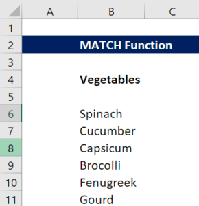
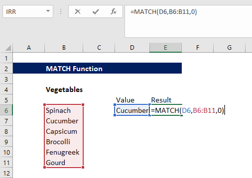
Example 1
Suppose we are given the following data:
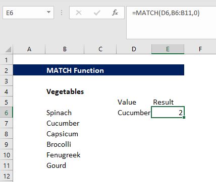
We can use the following formula to find the value for Cucumber.
We get the result below:
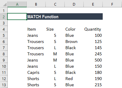
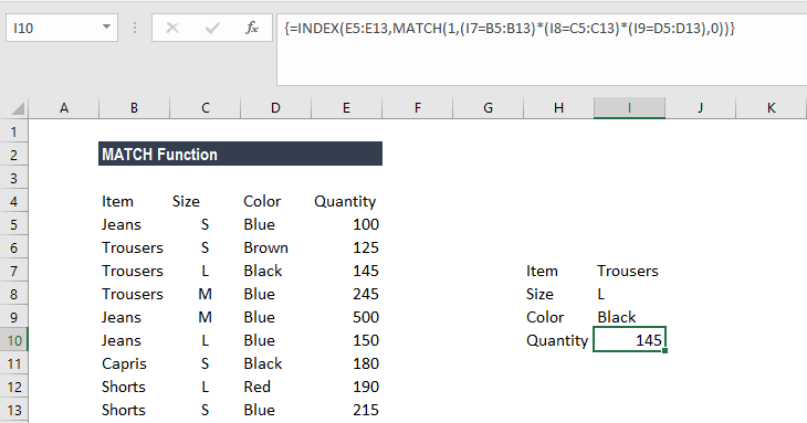
Example 2
Suppose we are given the following data:
Suppose we wish to find out the number of Trousers of a specific color. Here, we will use the INDEX or MATCH functions. The array formula to use is:
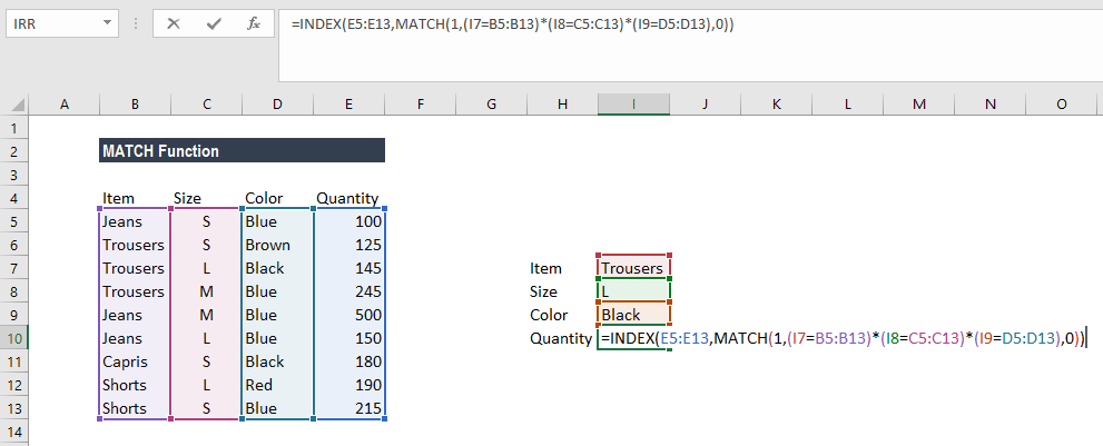
We need to create an array using CTRL + SHIFT + ENTER. We get the result below:
Things to Remember About the MATCH Function
- The MATCH function does not distinguish between uppercase and lowercase letters when matching text values.
- N/A! error – Occurs if the match function fails to find a match for the lookup_value.
- The function supports approximate and exact matching and wildcards (* or ?) for partial matches.
Click here to download the sample Excel file
Connect what you just learned to a clear career path with CFI’s role‑based courses and certification programs.
Additional Resources
Thank you for reading CFI’s guide to the MATCH Function. To learn more, check out these additional CFI resources:
- Excel Functions for Finance
- Advanced Excel Formulas Course
- Advanced Excel Formulas You Must Know
- Financial Analyst Program
Article Sources
Excel Tutorial
To master the art of Excel, check out CFI’s Excel Crash Course, which teaches you how to become an Excel power user. Learn the most important formulas, functions, and shortcuts to become confident in your financial analysis.

Launch CFI’s Excel Crash Course now to take your career to the next level and move up the ladder!


