NPER Function
Calculates the number of loan payment periods, given the periodic payment amount and (fixed) interest rate
What is the NPER Function?
The NPER Function[1] is categorized under Excel Financial functions. The function helps calculate the number of periods that are required to pay off a loan or reach an investment goal through regular periodic payments and at a fixed interest rate.
In financial analysis, we often wish to build a corporate fund. The NPER function will help us know the number of periods required to reach our target amount. It can also be used to get the number of payment periods for a loan that we wish to take.
Formula
=NPER(rate,pmt,pv,[fv],[type])
The NPER function uses the following arguments:
- Rate (required argument) – This is the interest rate per period.
- Pmt (required argument) – The payment made each period. Generally, it contains principal and interest but no other fees and taxes.
- Pv (required argument) – The present value, or the lump-sum amount that a series of future payments is worth right now.
- Fv (optional argument) – This is the future vale or the cash balance which we want at the end after the last payment is made. When omitted, it takes the value as zero.
- Type (optional argument) – Indicates when payments are due. If type is set to 0 or omitted, then payments are due at the end of the period. If set to 0, payments are due at the start of the period.
How to use the NPER Function in Excel?
As a worksheet function, NPER can be entered as part of a formula in a cell of a worksheet. To understand the uses of the function, let’s consider an example:
Example 1
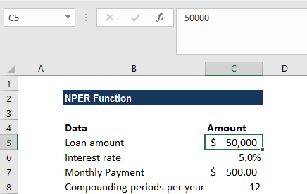
Let’s assume we need $50,000 and a loan will be given to us at a 5% interest rate, with a monthly payment of $500. Let’s now calculate the number of periods required to repay the loan.
The formula to be used would be:
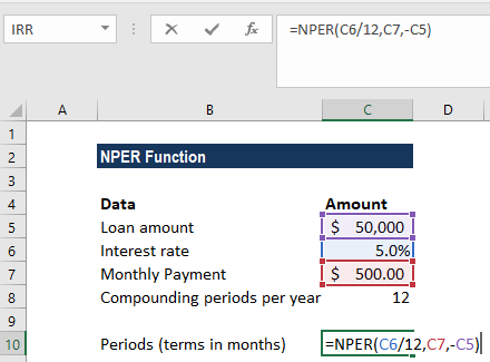
We get the result below:
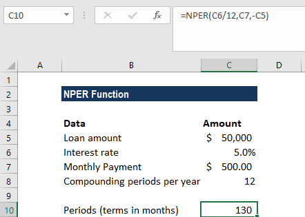
In the above example:
- We input the payment for the loan as a negative value, as it represents an outgoing payment.
- Payments are made monthly, so we needed to convert the annual interest rate of 5% into a monthly rate (=5%/12).
- We projected the future value as zero, and that the payment is to be made at the end of the month. Hence, the [fv] and [type] arguments can be omitted from the function call.
- The value returned by the function is in months. We then rounded the result to the nearest whole month, that is 130 months or 10 years, 10 months.
Example 2
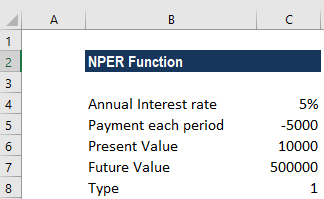
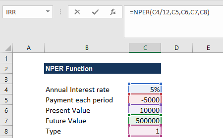
Let’s assume we wish to make an investment of $10,000 and want to earn $500,000. The annual interest rate is 5%. We will make additional monthly contributions of $5,000. Let’s now calculate the number of monthly investments required to earn $500,000.
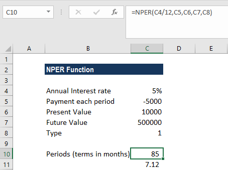
The formula to be used is:
We get the result below:
A few things to remember about the NPER Function:
- Remember that, in line with the cash flow convention, outgoing payments are represented by negative numbers and incoming cash flows by positive numbers.
- #NUM! error – Occurs if the stated future value will never be met or the supplied periodic interest rate and payments are insufficient. In such a scenario, we will need to increase the payment amount or increase the interest rate to achieve a valid result.
- #VALUE! error – Occurs if any of the given arguments are non-numeric values.
Click here to download the sample Excel file
Additional Resources
Thanks for reading CFI’s guide to important Excel functions! By taking the time to learn and master these functions, you’ll significantly speed up your financial analysis. To learn more, check out these additional CFI resources:
- Excel Functions for Finance
- Advanced Excel Formulas Course
- Advanced Excel Formulas You Must Know
- Excel Shortcuts for PC and Mac
- See all Excel resources
Article Sources
Excel Tutorial
To master the art of Excel, check out CFI’s Excel Crash Course, which teaches you how to become an Excel power user. Learn the most important formulas, functions, and shortcuts to become confident in your financial analysis.

Launch CFI’s Excel Crash Course now to take your career to the next level and move up the ladder!


