QUARTILE Function

What is the QUARTILE Function?

The QUARTILE Function[1] is categorized under Excel Statistical functions. The function will return the quartile of a given data set.

As a financial analyst, QUARTILE can be used to find out, for example, a specific percentage of incomes in a population. The function is very useful in revenue analysis.

Formula

=QUARTILE(array,quart)

The function uses the following arguments:

1. Array (required argument) – This is the array or cell range of numeric values for which we want the quartile value.
2. Quart (required argument) – This indicates which value will be returned. It is an integer between 0 and 4, representing the required quartile.

How to use the QUARTILE Function in Excel?

As a worksheet function, QUARTILE can be entered as part of a formula in a cell of a worksheet. To understand the uses of the function, let us consider a few examples:

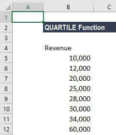
Example 1

Suppose we are given the following revenue figures:

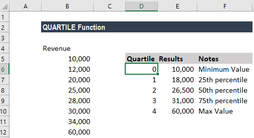
QUARTILE can return the minimum value, first quartile, second quartile, third quartile, and max value. The function accepts five values for the quart argument, as shown below:

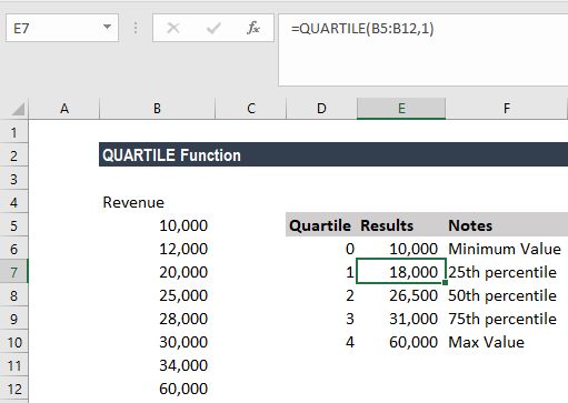
The formulas used are below:

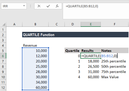
Similarly, we used 1 as quart argument for the 25^th percentile, 2 for the 50^th percentile, 3 for the 75^th percentile and 4 for max value.

We get the results below:

Example 2

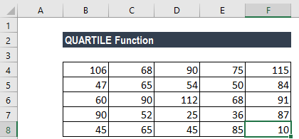
If we wish to highlight cells by quartile, we can apply conditional formatting with a formula that uses the QUARTILE function. Suppose we are given the following data:

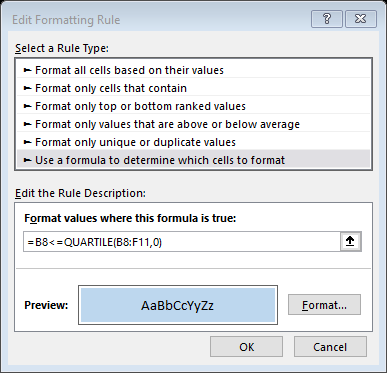
If we wish to highlight the minimum quartile, we can use conditional formatting. The formula to be used is:

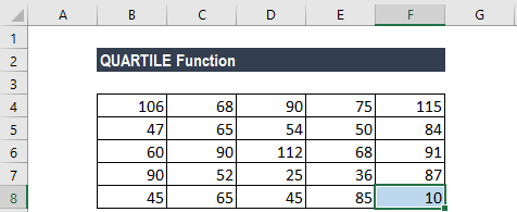
We get the result below:

If we want, we can highlight every cell based on the quartile it belongs to. For that, we will set four conditional formatting rules:

1. =A1>QUARTILE(A1:E5,3)
2. =A1>=QUARTILE(A1:E5,2)
3. =A1>=QUARTILE(A1:E5,1)
4. =A1>=QUARTILE(A1:E5,0)

The QUARTILE function is automatic and will calculate the 1st quartile with an input of 1, the 2nd quartile with an input of 2, and the 3rd quartile with an input of 3. With an input of 0, the function returns the minimum value in the data.

We need to arrange the conditional formatting rules so that they run in the same direction. The first rule highlights values greater than the 3rd quartile. The second rule highlights values greater than the 2nd quartile, the 3rd rule highlights data greater than the 1st quartile, and the last rule highlights data greater than the minimum value.

Things to remember about the QUARTILE Function 

1. #NUM! error – Occurs if either:
   1. The given value of quart is < 0 or > 4
   2. The given array is empty
2. #VALUE! error – Occurs if the given value of quart is non-numeric.

Click here to download the sample Excel file

Additional Resources

Thanks for reading CFI’s guide to important Excel functions! By taking the time to learn and master these functions, you’ll significantly improve your financial modeling. To learn more, check out these additional CFI resources:

• Excel Functions for Finance
• Financial Modeling Courses
• QUARTILE.INC Function
• STANDARDIZE Function
• See all Excel resources