ROWS Function

What is the ROWS Function?

The ROWS Function[1] is an Excel Lookup/Reference Function. The function is used to look up and provide the number of rows in each reference or array. Thus, the function, after receiving an Excel range, will return the number of rows that are contained within that range.

in financial analysis, we can use ROWS if we wish to count the number of rows in a given range.

Formula

=ROWS(array)

The ROWS function uses only one argument:

1. Array (required argument) – This is the reference to a range of cells or array or array formula for which we want the number of rows. The function will give us a numerical value.

How to use the ROWS Function in Excel?

To understand the uses of the ROWS function, let us consider a few examples:

Example 1

Let us see how the function works when we provide the following references:

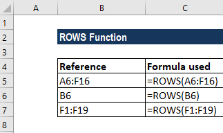
ROWS is useful if we wish to find out the number of rows in a range. The most basic formula used is =ROWS(rng).

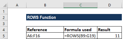
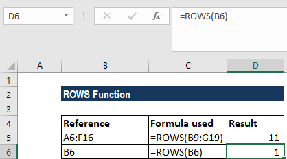
In the first reference, we used ROWS to get the number of columns from range B9:G19. We got the result as 11 as shown in the screenshot below:

The function counted the number of rows and returned a numerical value as the result.

When we gave the cell reference B6, it returned the result of 1 as only one reference was given.

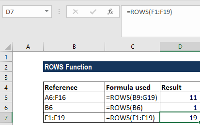
Lastly, when we provided the formula F1:F19, it counted the number of rows, which was 9, and returned the result accordingly.

In the ROWS function, Array can be an array, an array formula, or a reference to a single contiguous group of cells.

Example 2

If we wish to get the address of the first cell in a named range, we can use the ADDRESS function together with the ROW and COLUMN functions.

The formula to use is:

=ADDRESS(ROW(B5:D5)+ROWS(B5:D5)-1,COLUMN(B5:D5)+ROWS(B5:D5)-1)

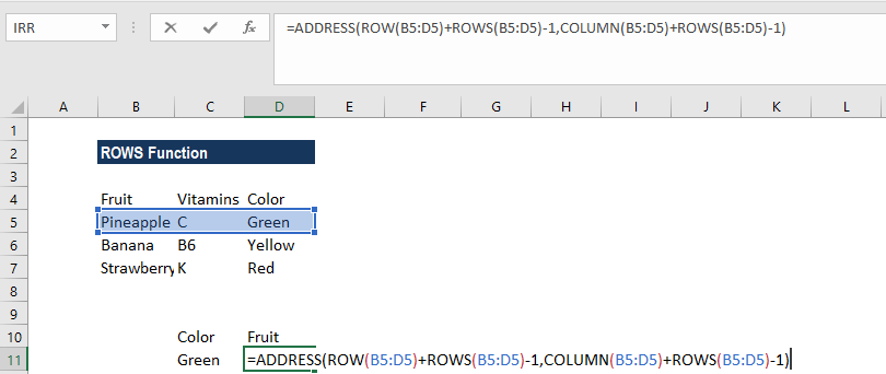
In the formula, the ADDRESS function builds an address based on a row and column number. Then, we use the ROW function to generate a list of row numbers, which are then shifted by adding ROWS(B5:D$)-1 so that the first item in the array is the last row number:

ROW(B5:D5)+ROWS(B5:D5)-1

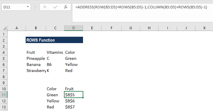
ADDRESS now collects and returns an array of addresses. If we enter the formula in a single cell, we just get the item from the array that is the address corresponding to the last cell in a range.

Example 3

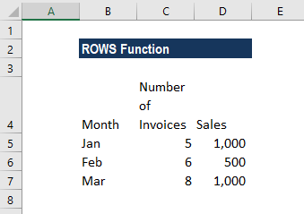
Now let’s see how to find out the last row in a range. The data given is as follows:

The formula used was =MIN(ROW(B5:D7))+ROWS(B5:D7)-1.

Using the formula above, we can get the last column that is in a range with a formula based on the ROW function.

When we give a single cell as a reference, the ROW function will return the row number for that particular reference. However, when we give a range that contains multiple rows, the ROW function will return an array that contains all ROW numbers for the given range.

If we wish to get only the first row number, we can use the MIN function to extract just the first row number, which will be the lowest number in the array.

Once the first row is given, we can just add the total rows in the range and subtract 1 to get the last row number.

We get the result below:

For a very large number of ranges, we can use the INDEX function instead of the MIN function. The formula will be =ROW(INDEX(range,1,1))+ROWS(range)-1.

Click here to download the sample Excel file

Additional Resources

Thanks for reading CFI’s guide to important Excel functions! By taking the time to learn and master these functions, you’ll significantly speed up your financial analysis. To learn more, check out these additional CFI resources:

• Advanced Excel Tutorial
• Advanced Excel Formulas
• Excel Keyboard Shortcuts
• CFI Financial Analyst Program
• See all Excel resources