TRANSPOSE Function
Flips the direction of a given range or array
What is the TRANSPOSE Function?
The TRANSPOSE Function[1] is categorized under Excel Lookup and Reference functions. It will flip the direction of a given range or array. The function will convert a horizontal range into a vertical range and vice versa.
In financial analysis, the TRANSPOSE function is useful in arranging data in our desired format.
Formula
=TRANSPOSE(array)
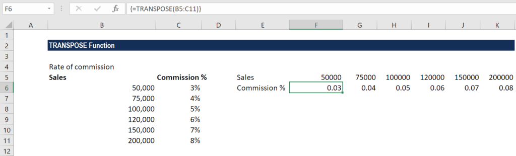
The array argument is a range of cells. The transposition of an array is created by using the first row of the array as the first column of the new array, the second row of the array as the second column of the new array, and so on.
To input an array formula in Excel, we need to:
- Highlight the range of cells for the function result;
- Type the function in the first cell of the range, and press CTRL-SHIFT-Enter.
How to use the TRANSPOSE Function in Excel?
TRANSPOSE is a built-in function that can be used as a worksheet function in Excel. To understand the use of TRANSPOSE, let us consider an example:
Example
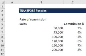
Suppose we are given the data below:
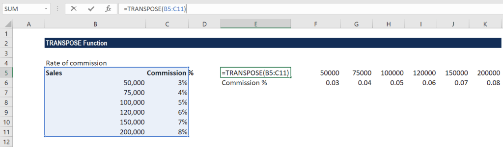
To transpose the data, we will use the following formula:
To enter the formula, follow the steps below:
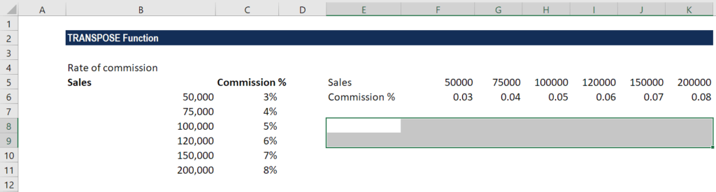
- First, we select some blank cells. They need to be of the same number of cells as the original set of cells but in the other direction. For example, there are eight cells here that are arranged vertically. So, we need to select eight horizontal cells, as shown below:
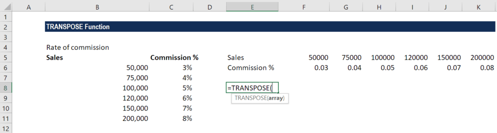
- The next step is to type =TRANSPOSE, as shown below:
- Next is to enter the range of the cells that we want to transpose. In this example, we want to transpose cells from A2 to B8. Finally, we will press CTRL+SHIFT+ENTER.
We get the results below:
When an array is transposed, the first row is used as the first column of the new array, the second row is used as the second column, and so on.
As mentioned above, we need to enter the TRANSPOSE function as an array formula that contains the same number of cells as the array using Control + Shift + Enter.
The new array must occupy the same number of rows as the source array has columns, and the same number of columns as the source array has rows.
For a one-off conversion, we can use Paste Special > TRANSPOSE.
Click here to download the sample Excel file
Additional Resources
Thanks for reading CFI’s guide to important Excel functions! By taking the time to learn and master these functions, you’ll significantly speed up your financial modeling. To learn more, check out these additional CFI resources:
- Excel for Finance
- Advanced Excel Formulas
- CODE Function
- COUNTIF Function
- SWITCH Function
- See all Excel resources
Article Sources
Excel Tutorial
To master the art of Excel, check out CFI’s Excel Crash Course, which teaches you how to become an Excel power user. Learn the most important formulas, functions, and shortcuts to become confident in your financial analysis.

Launch CFI’s Excel Crash Course now to take your career to the next level and move up the ladder!


