XMATCH Function
What is the XMATCH Function in Excel?
The XMATCH function in Microsoft Excel allows us to find the relative position within a data array of a specific entry. Microsoft introduced the XMATCH function in a 2019 update where it was described as a successor of the MATCH function. The MATCH function is one of the most popular Excel functions and is widely used in financial modeling. XMATCH offers more features than MATCH and is considerably easier and more intuitive to use.
MATCH Function in Excel
MATCH allows us to find the location of a specific entry within a data array. The MATCH function comes with the following syntax:
=MATCH(lookup_value,lookup_array,[match_type])
MATCH searches for the lookup value in the lookup array starting with the first cell in the array. MATCH only works with a single row or a single column, so the first cell is either the leftmost cell (when the lookup array is a single row) or the topmost cell (when the lookup array is a single column). A match type of 0 means that Excel only returns exact matches. A match type of -1 means that the position within the array of the first entry less than or equal to the lookup value is returned and a match type of 1 means that the position within the array of the first entry more than the lookup value is returned.
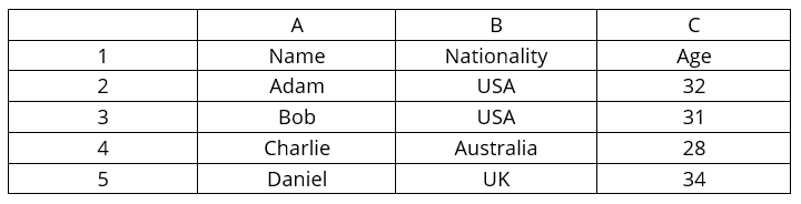
- =MATCH(Charlie,A2:A5,0): In this case, XMATCH searches for Charlie in the array A2:A5 starting with A2 and moving down towards A5. Here, the MATCH function will return 3 as output because Charlie is found in the 3rd cell of the array A2:A5.
- =MATCH(USA,A3:C3,0): In this case, XMATCH searches for USA in the array A3:C3 starting with A3 and moving right towards C3. Here, the MATCH function will return 2 as output because USA is found in the 2nd cell of the array A3:C3.
Understanding the XMATCH Function in Excel
XMATCH allows us to find the location of a specific entry within a data array. The syntax for the XMATCH function is as follows:
=XMATCH(lookup_value,lookup_array,[match_type],[search_type])
XMATCH searches for the lookup value in the lookup array starting with the first cell (unless specified) in the array. XMATCH only works with a single row or a single column, so the first cell (unless specified) is either the leftmost cell (when the lookup array is a single row) or the topmost cell (when the lookup array is a single column).
A match type of 0 means that Excel only returns exact matches. A match type of -1 means that the position within the array of the first entry less than or equal to the lookup value is returned and a match type of 1 means that the position within the array of the first entry more than the lookup value is returned. A match type of 2 means allows us to look for partial matches with unknown characters signposted with ‘?’ and unknown strings with ‘*’. Search type is set to 1 by default. A search type of -1 means that Excel searches the array backward.
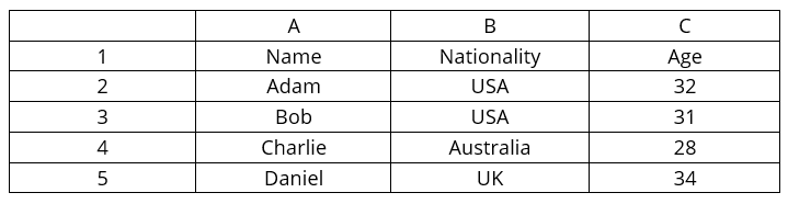
- =XMATCH(Charlie,A2:A5,0): XMATCH searches for Charlie in the array A2:A5 starting with A2 and moving down towards A5. Here, the XMATCH function will return 3 as output because Charlie is found in the third cell of the array A2:A5.
- =XMATCH(USA,A3:C3,0): XMATCH searches for USA in the array A3:C3 starting with A3 and moving right towards C3. Here, the XMATCH function will return 2 as output because USA is found in the second cell of the array A3:C3.
- =XMATCH(B?B,A2:A5,2): XMATCH searches for B?B in the array A2:A5 starting with A2 and moving down towards A5. In this case XMATCH returns 2. However, if the entry in A2 were Bab, Bbb, Bcb… etc, XMATCH would’ve returned 1.
- =XMATCH(Au*,B2:B5,2): XMATCH searches for Au* in the array B2:B5 starting with B2 and moving down towards B5. Here, XMATCH returns 3. However, if the entry in B2 were Austria, XMATCH would’ve returned 1.
- =XMATCH(Charlie,A2:A5,0): XMATCH searches for Charlie in the array A2:A5 starting with A5 and moving down towards A2. Here, the XMATCH function will return 2 as output because Charlie is found in the second cell of the array A2:A5 when searching from below.
Illustrative Example
A financial analyst wants to find out how different currencies are doing against the US dollar. The analyst is given the following spreadsheet:

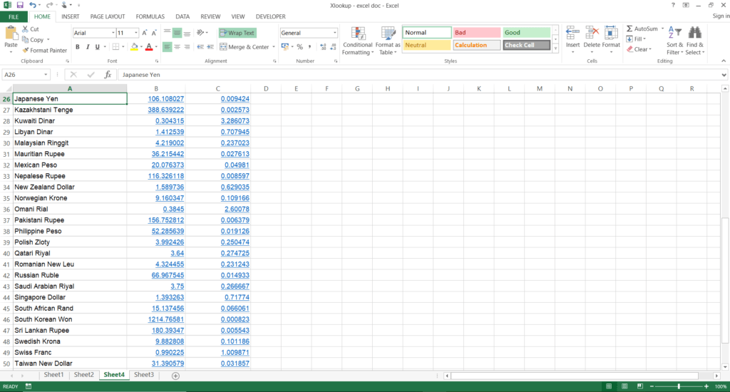

The analyst wants to answer two questions: How many currencies are stronger than the US dollar in absolute terms, i.e., 1x= more than $1 and how are the GBP/USD and EUR/USD rankings in absolute terms? The analyst first needs to sort the data in ascending order using the second column (inverse exchange rate).

Next, the analyst can use the XMATCH function to answer both questions.
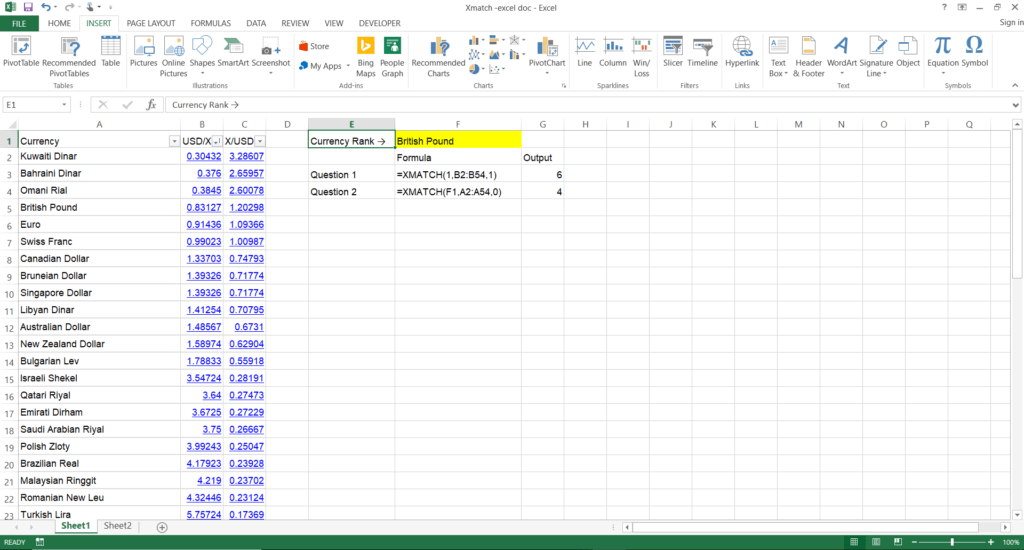

There are six currencies that are stronger than the US dollar in absolute terms, i.e., 1x= more than $1. The British pound and the euro rank fourth and fifth, respectively, among currencies that are stronger than the US dollar in absolute terms.
Additional Resources
CFI is the official provider of the Financial Modeling and Valuation Analyst (FMVA)™ certification program, designed to transform anyone into a world-class financial analyst.
To keep learning and developing your knowledge of financial analysis, we highly recommend the additional resources below:
Excel Tutorial
To master the art of Excel, check out CFI’s Excel Crash Course, which teaches you how to become an Excel power user. Learn the most important formulas, functions, and shortcuts to become confident in your financial analysis.

Launch CFI’s Excel Crash Course now to take your career to the next level and move up the ladder!


