CHISQ.TEST Function in Excel
Calculates the chi-square distribution of two provided datasets
What is the CHISQ.TEST Function?
The CHISQ.TEST function[1] is categorized under Excel statistical functions. It will calculate the chi-square distribution of two provided datasets, specifically, the observed and expected frequencies. The function helps us understand whether the differences between the two sets is simply due to sampling error, or not.
In financial analysis, CHISQ.TEST can be used to find out the variations in observed and expected frequencies, e.g., defective items produced by machines A and B. Comparing the observed and expected frequencies with this function will help us understand if sampling error caused the difference in the two frequencies.
The chi-square distribution is given by the formula:
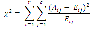
where:
Aij – Actual frequency in the i’th row and j’th column
Eij – Expected frequency in the i’th row and j’th column
r – Number of rows
c – Number of columns
The chi-square test gives an indication of whether the value of the chi-square distribution, for independent sets of data, is likely to happen by chance alone.
CHISQ.TEST Formula
=CHISQ.TEST(actual_range,expected_range)
The CHISQ.TEST uses the following arguments:
- Actual_range (required argument) – This is the range of data containing observations that are to be tested against expected values. It is an array of observed frequencies.
- Expected_range (required argument) – This is the range of data that contains the ratio of the product of row totals and column totals to the grand total. It is an array of expected frequencies.
When providing the arguments, it is necessary that the actual_range and the expected_range arrays are of equal dimensions.
To learn more, launch our free Excel crash course now!
How to Use the CHISQ.TEST Function
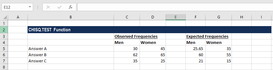
To understand the uses of the CHISQ.TEST function, let us consider an example.
Suppose we are given the following data:
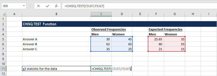
The formula for calculating the chi-square test for the independence of the datasets above is:
We get the result below:
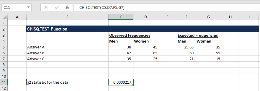
Generally, a probability of 0.05 or less is considered to be significant. Therefore, the returned value above, 0.0000217, indicates a significant difference between the observed and the expected frequencies, which is unlikely to be due to sampling error.
A few notes about the CHISQ.TEST function
- #DIV/0! error – Occurs when any of the values provided in expected_range is zero.
- #N/A error – Occurs when either:
- The data arrays provided are of different dimensions; or
- The data arrays provided contain only one value. That is, the length and width are equal to 1.
- #NUM! error – Occurs when any of the values in the expected range is negative.
- The CHISQ.TEST function was introduced in Excel 2010 and hence is unavailable in earlier versions. It is an updated version of the CHITEST function.
Additional Resources
Advanced Excel Formulas You Must Know
Article Sources
Excel Tutorial
To master the art of Excel, check out CFI’s Excel Crash Course, which teaches you how to become an Excel power user. Learn the most important formulas, functions, and shortcuts to become confident in your financial analysis.

Launch CFI’s Excel Crash Course now to take your career to the next level and move up the ladder!


