ISERROR Function
Returns TRUE if the given value is an error and vice versa
What is the ISERROR Excel Function?
The ISERROR Excel Function[1] is categorized under Information functions. The function will return TRUE if the given value is an error and FALSE if it is not. It works on errors – #N/A, #VALUE!, #REF!, #DIV/0!, #NUM!, #NAME? or #NULL.
ISERROR is used in combination with the IF function to identify a potential formula error and display other formulas or text strings in message form or blanks. It can also be used with the IF function to display a custom message or perform some other calculation if an error is found.
In financial analysis, we need to deal with formulas and data. Often, our spreadsheet contains a large number of formulas and they sometimes don’t work properly to perform calculations as required when an error is encountered. Just like the ISERR function, ISERROR, in combination with the IF function, can be used to default a cell’s value when an error is encountered. It allows our formulas to work and evaluate data properly without requiring the user’s intervention.
Formula
=ISERROR(value)
The ISERROR function uses the following argument:
- Value (required argument) – This is the expression or value that needs to be tested. It is generally provided as a cell address.
How to use the ISERROR Excel Function?
To understand the uses of the ISERROR Excel function, let’s consider a few examples:
Example 1
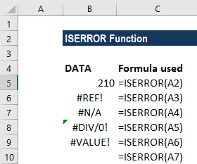
Let’s see the results from the function when we provide the following data:
| Data | Formula | Result | Remarks |
|---|---|---|---|
| 210 | =ISERR(210) | FALSE | As there is no error, so FALSE |
| #REF! | =ISERR(#REF!) | TRUE | TRUE, as it is an error |
| #N/A | =ISERR(#NA) | TRUE | Unlike ISERR, it does take the error N/A |
| 25/0 | =ISERR(25/0) | TRUE | TRUE, as the formula is an error |
| #VALUE! | =ISERR(#VALUE!) | TRUE | TRUE, as it is an error |
| =ISERR() | FALSE | No error, so FALSE |
Example 2
If we wish to count the number of cells that contain errors, we can use the ISERROR function, wrapped in the SUMPRODUCT function.
Suppose we are given the following data:
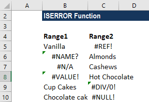
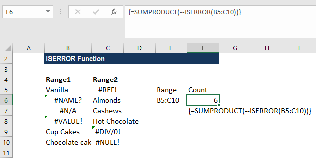
Using the formula =SUMPRODUCT(–ISERROR(B5:C10)), we can get the count of cells with an error, as shown below.
In the above formula:
- The SUMPRODUCT function accepted one or more arrays and calculated the sum of the products of corresponding numbers.
- ISERROR now evaluates each of the cells in the given range. The result will be TRUE,FALSE,FALSE,FALSE,TRUE,TRUE,FALSE,TRUE,TRUE,TRUE,FALSE,FALSE.
- As we used double unary, the results TRUE/FALSE were transformed to 0 and 1. It made the results look like {0,1,1,1,0,0,1,0,0,0,1,1}.
- SUMPRODUCT now sums the items in the given array and returns the total, which, in the example, is the number 6.
- As an alternative, the SUM function can be used. The formula to use will be =SUM(–ISERROR(range)). Remember to put the formula in an array. For the array, we need to press Control + Shift + Enter instead of just Enter.
Example 3
If we wish to provide a custom message, for example, instead of getting #DIV/0 error, we want the value to be 0. We can use the formula =IF(ISERROR(A4/B4),0,A4/B4) instead of A4/B4.
Suppose we are given the following data:
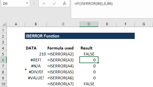
Instead of TRUE, if we wish to enter the value 0, the formula to use will be =IF(ISERROR(B6),0,B6) and not B6, as shown below:
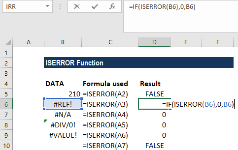
We get the result below:
Click here to download the sample Excel file
Additional Resources
Thanks for reading CFI’s guide to important Excel functions! By taking the time to learn and master these functions, you’ll significantly speed up your financial analysis. To learn more, check out these additional CFI resources:
- Excel Functions for Finance
- Advanced Excel Formulas You Must Know
- Excel Shortcuts for PC and Mac
- DSUM Function
- See all Excel resources
Article Sources
Excel Tutorial
To master the art of Excel, check out CFI’s Excel Crash Course, which teaches you how to become an Excel power user. Learn the most important formulas, functions, and shortcuts to become confident in your financial analysis.

Launch CFI’s Excel Crash Course now to take your career to the next level and move up the ladder!


