SUBTOTAL Function in Excel
Returns an aggregate result for data provided
What is the SUBTOTAL Function in Excel?
The SUBTOTAL Function[1]in Excel allows users to create groups and then perform various other Excel functions such as SUM, COUNT, AVERAGE, PRODUCT, MAX, etc. Thus, the SUBTOTAL function in Excel helps in analyzing the data provided.
Formula
SUBTOTAL = (method, range1, [range2 …range_n])
Where method is the type of subtotal you wish to obtain
Range1,range2…range_n is the range of cells you wish to subtotal
Why do we need to use SUBTOTALS?
Sometimes, we need data based on different categories. SUBTOTALS help us to get the totals of several columns of data broken down into various categories.
For example, let’s consider garment products of different sizes manufactured. The SUBTOTAL function will help you to get a count of different sizes in your warehouse.
To learn more, launch our free Excel crash course now!
Download the Free Template
How to use the SUBTOTAL Function in Excel?
There are two steps to follow when we wish to use the SUBTOTAL function. These are:
- Formatting and sorting of the provided Excel data.
- Applying SUBTOTAL to the table.
Let’s understand this Excel function with the help of an example. We use data provided by a garment manufacturer. He manufactures T-shirts of five different colors, i.e., White, Black, Pink, Green, and Beige. He produces these T-shirts in seven different sizes, i.e. 2, 4, 6, 8, 10, 12, 14. The relevant data are below:
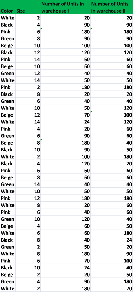
The warehouse manager provides random data. Now for the analysis, we need to get the total number of T-shirts of each color lying in the warehouse.
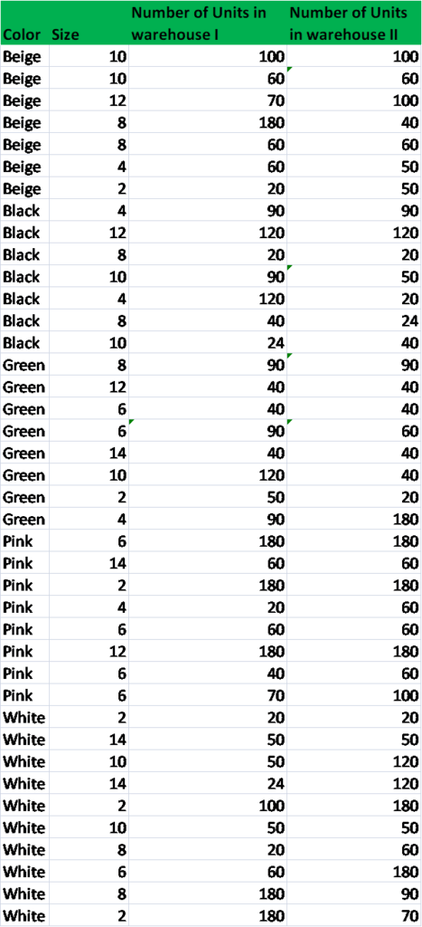
Step 1
First, we need to sort the worksheet on the basis of data we need to subtotal. As we need to get the subtotals of T-shirts by colors, we will sort it accordingly.
To do that, we can use the SORT function under the Data tab.
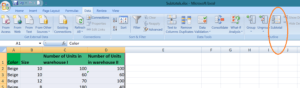
Step 2
The next step would be to apply the SUBTOTAL function. This can be done as shown below:
Select the Data tab, and click on SUBTOTAL.
When we click on it, the Subtotal dialogue box will appear as shown below:
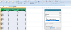
Now, click the drop-down arrow for the “At each change in: field.” We can now select the column we wish to subtotal. In our example, we’ll select Color.
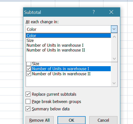
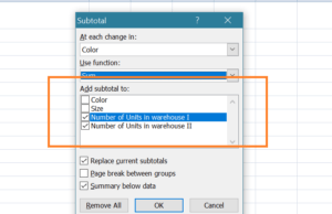
Next, we need to click the drop-down arrow for the “Use function: field.” This will help us select the function we wish to use. There are 11 available functions. We need to choose depending on our requirements. In our example, we’ll select SUM to find out the total number of T-shirts lying in each warehouse.

Next, we move to “Add subtotal to: field.” Here we need to select the column where we require the calculated subtotal to appear. In our example, we’ll select Number of Units in Warehouse I and Warehouse II.
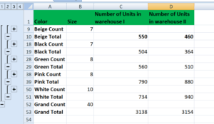
After that, we need to click OK and we will get the following results:

As we can see in the screenshot above, the subtotals are inserted as new rows below each Group. When we create subtotals, our worksheet is divided into different levels. Depending on the information you wish to display in the worksheet, you can switch between these levels.
The level buttons in our example are images of buttons for Levels 1, 2, 3, which can be seen on the left side of the worksheet. Now suppose I just want to see the total T-shirts lying in the warehouse of different colors, we can click on Level 2.
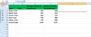
If we click on the highest level (Level 3), we will get all the details.
To learn more, launch our free Excel crash course now!
Video Tutorial – SUBTOTAL Function in Excel
To learn more about using the SUBTOTAL Function in Excel, check out the video below:
Tips for the SUBTOTAL function
Tip #1
Let’s assume, we wish to ensure that all colors of T-shirts are available in all sizes in either of the warehouses. We can follow these steps:
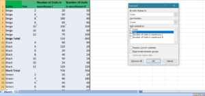
Step 1: Click on Subtotal. Remember we are adding one more criterion to our current Subtotal data.
Now,
Step 2: Select COUNT from the drop-down menu, and Size from the “Add subtotal field to.” After that, uncheck the “Replace current subtotals.” Once you click OK, you will get the following data:
This will help us ensure that the count for different sizes and we can sort data in such a manner that the repetitions are not there.
Tip #2
Always sort data by column we will use to subtotal.
Tip #3
Remember that each column we wish to subtotal includes a label in the first row.
Tip #4
If you wish to put a summary of the data, uncheck the box “Summary below the data when inserting Subtotal.”
Free Excel Course
Check out our Free Excel Crash Course to learn more about Excel functions using your own personal instructor. Master Excel functions to create more sophisticated financial analysis and modeling towards building a successful career as a financial analyst.
Additional Resources
Thanks for reading CFI’s guide to important Excel functions! By taking the time to learn and master these functions, you’ll significantly speed up your financial analysis. To learn more, check out these additional CFI resources:
- Excel Functions for Finance
- CUMPRINC Function
- PRICE Function
- PRICEDISC Function
- WEIBULL.DIST Function
- See all Excel resources
Article Sources
Excel Tutorial
To master the art of Excel, check out CFI’s Excel Crash Course, which teaches you how to become an Excel power user. Learn the most important formulas, functions, and shortcuts to become confident in your financial analysis.

Launch CFI’s Excel Crash Course now to take your career to the next level and move up the ladder!


