IFERROR Function

What is the IFERROR Function?

IFERROR[1] is a function found under the Excel Logical Functions category. IFERROR belongs to a group of error-checking functions such as ISERR, ISERROR, IFERROR, and ISNA. The function will return a customized output – usually set to a string of text –  whenever the evaluation of the formula is an error.

In financial analysis, we need to deal with formulas and data. Often, we may get errors in cells with a formula. IFERROR is often used for error handling/capture. It handles errors such as #N/A, #VALUE!, #REF!, #DIV/0!, #NUM! #NAME? or #NULL!.

For example, the formula in C2 is A2/B2, where:

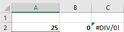
Instead of the resulting error, we can use IFERROR to return a customized message such as “Invalid input.”

Formula

=IFERROR(value,value_if_error)

The IFERROR Function uses the following arguments:

1. Value (required argument) – This is the expression or value that needs to be tested. It is generally provided as a cell address.
2. Value_if_error (required argument) – The value that will be returned if the formula evaluates to an error.

To learn more, launch our free Excel crash course now!

How to use IFERROR in Excel

As a worksheet function, IFERROR can be entered as part of a formula in a cell of a worksheet.

To understand the uses of the function, let’s consider a few examples:

IFERROR – Error Capturing

Suppose we are given the following data:

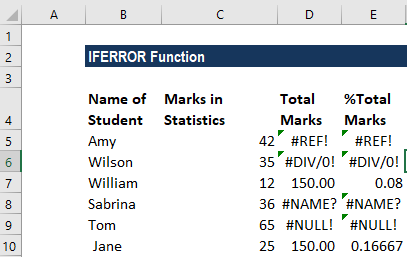
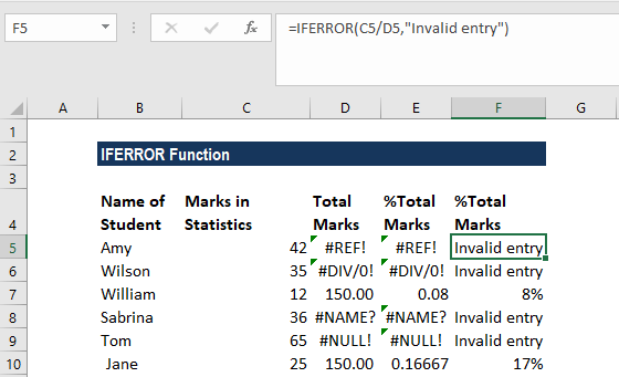
Using the IFERROR formula, we can remove these errors. We will put a customized message – “Invalid data.” The formula to be used is:

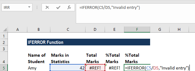
We will get the result below:

IFERROR + VLOOKUP Function

A very common use of IFERROR function is with the VLOOKUP function, where it is used to point out values that can’t be found.

Suppose we operate a restaurant and maintain an inventory of a few vegetables and fruits. Now we compare that inventory with the list of items we want according to the day’s menu. The results look like this:

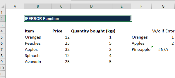
Instead of the #N/A error message, we can input a customized message. That looks better when we are using a long list.

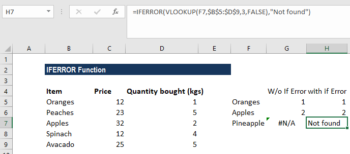
The formula to use will be:

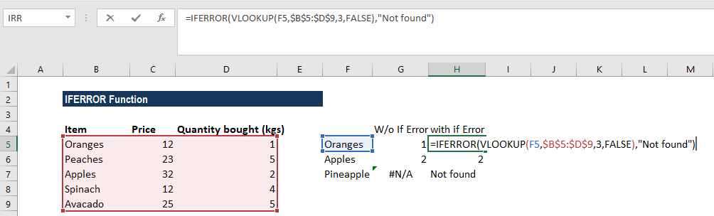
We get the result below:

Suppose we are given monthly sales data for the first quarter. We create three worksheets – Jan, Feb, and March.

Now we wish to find out the sales figures from certain order ids. As data would be derived by VLOOKUP from three sheets, using IFERROR, we can use the following formula:

=IFERROR(VLOOKUP(A2,’JAN’!A2:B5,2,0),IFERROR(VLOOKUP(A2,’FEB’!A2:B5,2,0),IFERROR(VLOOKUP(A2,’MAR’!A2:B5,2,0),”not found”))) 

Things to remember about the IFERROR Function

1. The IFERROR Function was introduced in Excel 2007 and is available in all subsequent Excel versions.
2. If the value argument is a blank cell, it is treated as an empty string (”’) and not an error.
3. If the value is an array formula, IFERROR returns an array of results for each cell in the range specified in value.

Click here to download the sample Excel file

Additional Resources

Thank you for reading CFI’s guide to IFERROR Function. To learn more, check out these additional CFI resources:

• Excel Functions for Finance
• Advanced Excel Formulas Course
• ISERR Function
• NA Function
• See all Excel resources