SUMIF Function

What is the SUMIF Function?

The SUMIF Function[1] is categorized under Excel Math and Trigonometry functions. It will sum up cells that meet the given criteria. The criteria are based on dates, numbers, and text. It supports logical operators such as (>, <, <>, =) and also wildcards (*, ?). This guide to the SUMIF Excel function will show you how to use it, step-by-step.

As a financial analyst, SUMIF is a frequently used function. Suppose we are given a table listing the consignments of vegetables from different suppliers. The names of the vegetable, names of suppliers, and quantity are in column A, column B, and column C, respectively. In such a scenario, we can use the SUMIF function to find out the sum of the amount related to a particular vegetable from a specific supplier.

Formula

=SUMIF(range, criteria, [sum_range])

The formula uses the following arguments:

1. Range (required argument) – This is the range of cells that we want to apply the criteria against.
2. Criteria (required argument) – This is the criteria which are used to determine which cells need to be added.

When we provide the criteria argument, it can either be:

• A numeric value (which may be an integer, decimal, date, time, or logical value) (e.g. 10, 01/01/2018, TRUE) or
• A text string (e.g. “Text”, “Thursday”) or
• An expression (e.g. “>12”, “<>0”).

3. Sum_range (optional argument) – This is an array of numeric values (or cells containing numeric values) that are to be added together if the corresponding range entry satisfies the supplied criteria. If the [sum_range] argument is omitted, the values from the range argument are summed instead.

How to use the SUMIF Excel Function

To understand the uses of the SUMIF function, let’s consider a few examples:

Example 1

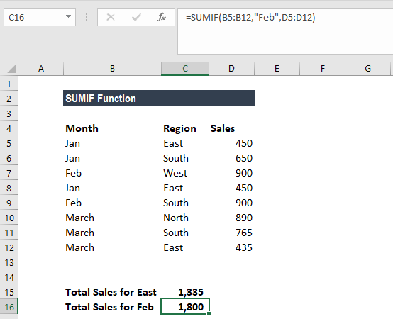
Suppose we are given the following data:

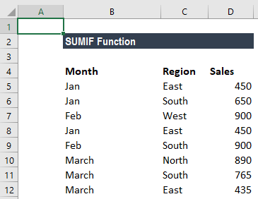
We wish to find total sales for the East region and the total sales for February. The formula to use to get the total sales for East is:

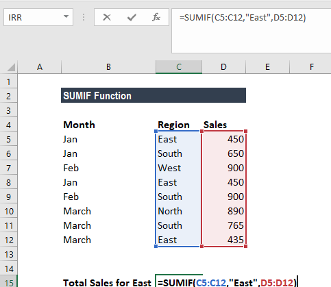
Text criteria, or criteria that includes math symbols, must be enclosed in double quotation marks (” “).

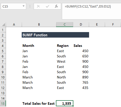
We get the result below:

The formula for total sales in February is:

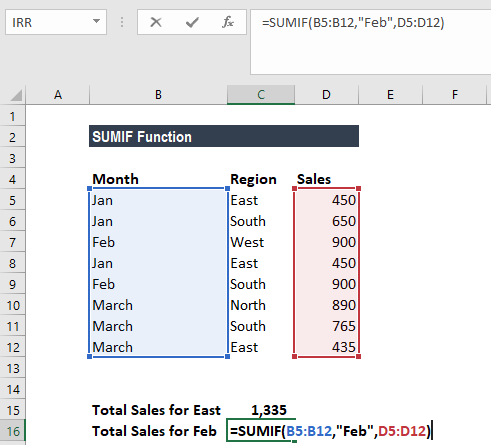
We get the result below:

A few notes about the SUMIF Excel Function 

1. #VALUE! error – Occurs when the criteria provided is a text string that is more than 255 characters long.
2. When sum_range is omitted, the cells in range will be summed.
3.  The following wildcards can be used in text-related criteria:
   • ? – matches any single character
   • * – matches any sequence of characters
4. To find a literal question mark or asterisk, use a tilde (~) in front of the question mark or asterisk (i.e. ~?, ~*).

Click here to download the sample Excel file

Additional Resources

Thanks for reading CFI’s guide to important Excel functions! By taking the time to learn and master these functions, you’ll significantly speed up your financial analysis. To learn more, check out these additional CFI resources:

• Excel Functions for Finance
• Advanced Excel Formulas Course
• Advanced Excel Formulas You Must Know
• Excel Shortcuts for PC and Mac
• See all Excel resources