TRUNC Function

What is the TRUNC Function?

The TRUNC Function[1] is an Excel Math and Trigonometry function. It removes the fractional part of a number and, thus, truncates a number to an integer. It was introduced in MS Excel 2007.

In financial analysis, the function can be used to truncate a number to a given precision. It is also useful for extracting dates from date and time values.

Formula

=TRUNC(number,[num_digits])

The TRUNC function uses the following arguments:

1. Number (required argument) – This is the number we wish to truncate.
2. Num_digits (optional argument) – This is a number that specifies the precision of the truncation. If kept blank, it will take 0 as the default value.

Now, if the num_digits argument is:

1. A positive value that is greater than zero, it specifies the number of digits to the right of the decimal point.
2. Equal to zero, it specifies the rounding to the nearest integer.
3. A negative value that is less than zero, it specifies the number of digits to the left of the decimal point.

How to use the TRUNC Function in Excel?

To understand the uses of the TRUNC function, let’s consider a few examples:

Example 1

Suppose we are given the following data:

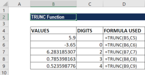
We get the results below:

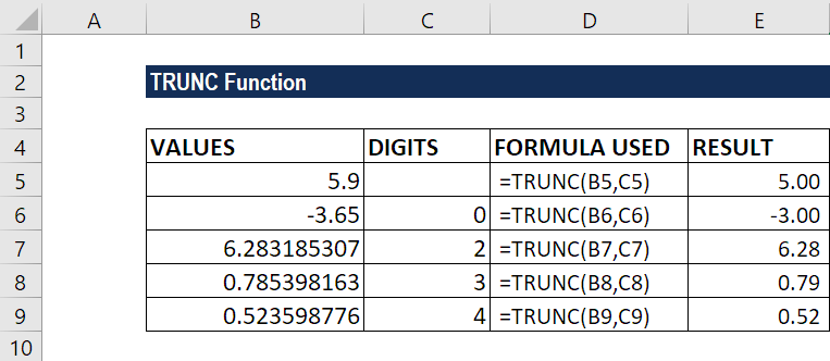
The TRUNC function does not round off but simply truncates a number as specified. The function can also be used to return a set number of decimal places without rounding off using the num_digits argument. For example, =TRUNC(PI(),2) will return Pi value truncated to two decimal digits, which is 3.14, and =TRUNC(PI(),3) will return Pi value truncated to three decimal places, which is 3.141.

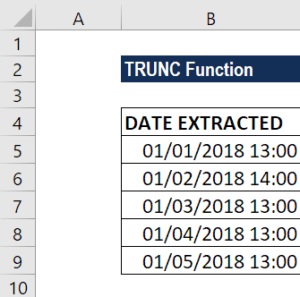
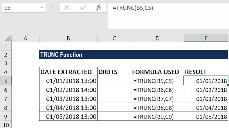
Example 2

Suppose we are given the following dates and time from an external source:

The formula to extract the date is:

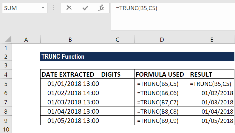
We get the result below:

Things to remember about the TRUNC Function

1. TRUNC and INT are similar functions because they both return the integer part of a number. The difference is that TRUNC merely truncates a number, but INT rounds off a number.

However, for positive numbers, as well as when TRUNC uses 0 as the default for num_digits, both functions will return the same results.

With negative numbers, the results can be different. =INT(-2.1) returns -3, because INT rounds down to the lower integer. =TRUNC(-2.1) returns -2.

Click here to download the sample Excel file

Additional Resources

Thanks for reading CFI’s guide to the Excel TRUNC function. By taking the time to learn and master these Excel functions, you’ll significantly speed up your financial analysis. To learn more, check out these additional CFI resources:

• Excel Functions for Finance
• Advanced Excel Formulas Course
• Advanced Excel Formulas You Must Know
• Excel Shortcuts for PC and Mac
• See all Excel resources