Get Certified for
Business Intelligence (BIDA®)
Develop analytical superpowers by learning how to use programming and data analytics tools such as VBA, Python, Tableau, Power BI, Power Query, and more.
A look at means, weighted averages and frequency distributions
A solid understanding of statistics is crucially important in helping us better understand finance. Moreover, statistics concepts can help investors monitor the performance of their investment portfolios, make better investment decisions, and understand market trends.

The mean return on investment of a portfolio is an arithmetic average of returns achieved over specified time periods. The statistic can easily be calculated by adding together all returns for a portfolio per unit time and dividing by the number of observations.
For example, consider a portfolio that has achieved the following returns: (Q1) +10%, (Q2) -3%, (Q3) 8%, (Q4) 12% and (Q5) -7% over 5 quarters. The mean return on investment would be calculated as follows:
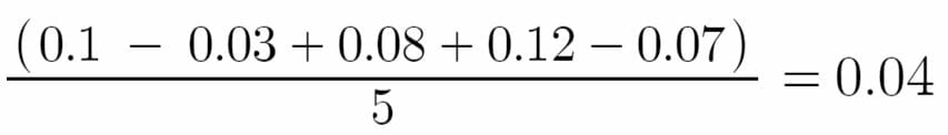
This would give us a mean return of 4% over the five quarters.
The Geometric mean statistic is an alternative method of calculating an average return on an investment portfolio. The equation for calculating geometric mean is:

Where:
R – the return realized in a specified uniform time period
n – the number of observations.
Using the information from the arithmetic mean example, we get the following:

Using the geometric mean method, we obtain a return of 3.72%.
The median statistic is the middle value in a set of observations. Using the numbers from the previous example, we can arrange them in the following ascending order: (Q5) -7%, (Q2) -3%, (Q3) 8%(Q1) +10%, (Q4) 12%.
The middle value in this series is 8%, achieved in Q3. Therefore, the mean return of the portfolio would be 8%.
The weighted average return statistic takes into account how much of a given portfolio is invested in a particular asset. The formula to calculate weighted average is:

Where:
R – returns for a particular asset or asset class
W – the percentage weight of that particular asset in the portfolio
Let’s look at the following portfolio returns:
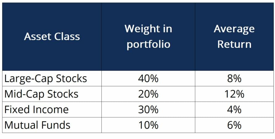
In this table, the average return could be expressed as an arithmetic mean, geometric mean or median of returns for the asset class over a certain period of time. Using the formula provided above, we can calculate the weighted average return to be:

This would provide us with a weighted average return of 7.4%.
Relative and cumulative frequencies are statistics that can be used to obtain a more concrete understanding of how an investment portfolio is performing. Relative frequency counts the number of observations that fall within a certain range (or “bucket”) of returns, while cumulative frequency counts the total number of observations that fall in all buckets up to a certain point. The table below illustrates these concepts:
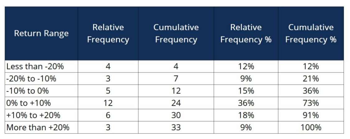
In this example:
Return Range – refers to the ranges of returns we want to calculate relative and cumulative frequencies for.
Relative Frequency – is the number of assets in the portfolio that fall under the specified return ranges (ex., the portfolio contains 12 assets that have produced returns of 0 to +10%).
Cumulative Frequency – is the sum of all observations that fall in the current return range or in previous return ranges (ex., the portfolio contains 30 assets that have produced returns of 20% or less).
Relative Frequency % – is the percentage of assets that fall within a specific return range (ex., 9% of the assets in the portfolio have produced returns between -20% and -10%).
Cumulative Frequency % – is the percentage of all assets that fall within a specific return range or below (ex., 73% of the assets in the portfolio have produced a return of +10% or less). The difference between the cumulative frequency and 100% will tell us how many assets in the portfolio have achieved a certain return or better. For example, 27% (100%-73%) of the portfolio has produced returns of more than +10%.
Hence, relative and cumulative frequencies are useful in better understanding how an investment portfolio is performing.
Frequency distribution charts, or histograms, are essentially graphical representations of the cumulative frequency numbers. The histogram below is based on the numbers provided in the example above.
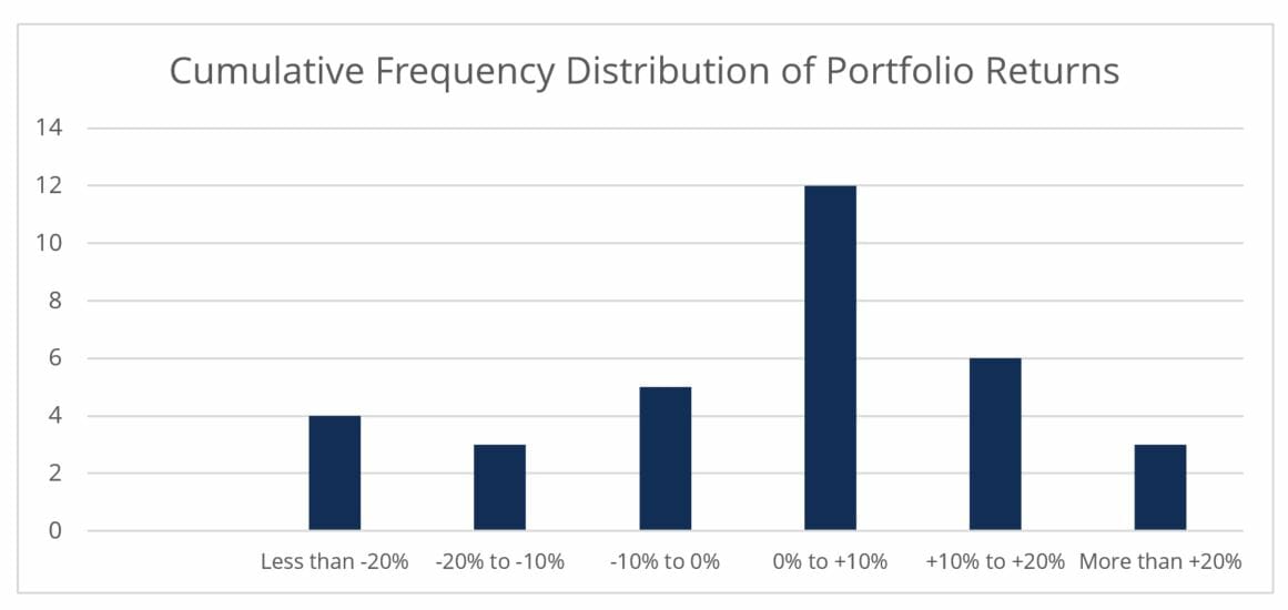
Each column represents the number of assets that fell into the various return ranges. Here again, this interpretation of data provides a brief portfolio-wide snapshot of returns.
CFI offers the Business Intelligence & Data Analyst (BIDA®) certification program for those looking to take their careers to the next level. To learn more about related topics, check out the following resources:


