Capital Allocation Line (CAL) and Optimal Portfolio

Capital Allocation Line (CAL) and Optimal Portfolio

The Capital Allocation Line (CAL) is a line that graphically depicts the risk-and-reward profile of assets, and can be used to find the optimal portfolio. The process to construct the CAL for a collection of portfolios is described below. 

Portfolio expected return and variance

For the sake of simplicity, we will construct a portfolio with only two risky assets.

The portfolio’s expected return is a weighted average of its individual assets’ expected returns, and is calculated as:

E(Rp) = w₁E(R₁) + w₂E(R₂)

Where w₁, w₂ are the respective weights for the two assets, and E(R₁), E(R₂) are the respective expected returns.

Levels of variance translate directly with levels of risk; higher variance means higher levels of risk and vice versa. The variance of a portfolio is not just the weighted average of the variance of individual assets but also depends on the covariance and correlation of the two assets. The formula for portfolio variance is given as:

Var(R_p) = w²₁Var(R₁) + w²₂Var(R₂) + 2w₁w₂Cov(R₁, R₂)

Where Cov(R₁, R₂) represents the covariance of the two asset returns. Alternatively, the formula can be written as:

σ²_p = w²₁σ²₁ + w²₂σ²₂ + 2ρ(R₁, R₂) w₁w₂σ₁σ₂, using ρ(R₁, R₂), the correlation of R₁ and R₂.

The conversion between correlation and covariance is given as: ρ(R₁, R₂) = Cov(R₁, R₂)/ σ₁σ₂.

The variance of portfolio return is greater when the covariance of the two assets is positive, and less when negative. Since variance represents risk, the portfolio risk is lower when its asset components possess negative covariance. Diversification is a technique that minimizes portfolio risk by investing in assets with negative covariance.

In practice, we do not know the returns and standard deviations of individual assets, but we can estimate these values based on these assets’ historical values.

The efficient frontier

A portfolio frontier is a graph that maps out all possible portfolios with different asset weight combinations, with levels of portfolio standard deviation graphed on the x-axis and portfolio expected return on the y-axis.

To construct a portfolio frontier, we first assign values for E(R₁), E(R₂), stdev(R₁), stdev(R₂), and ρ(R₁, R₂). Using the above formulas, we then calculate the portfolio expected return and variance for each possible asset weight combinations (w₂=1-w₁). This process can be done easily in Microsoft Excel, as shown in the example below:

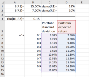
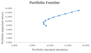
We then use the scatter chart with smooth lines to plot the portfolio’s expected return and standard deviation. The result is shown on the graph below, where each dot on the plot represents a portfolio constructed under an asset weight combination.

So how do we know which portfolios are attractive to investors? To answer this, we introduce the concept of mean-variance criterion, which states that Portfolio A dominates Portfolio B if E(R_A) ≥ E(R_B) and σ_A ≤ σ_B (i.e. portfolio A offers a higher expected return and lower risk than portfolio B). If such is the case, then investors would prefer A to B.

From the graph, we can infer that portfolios on the downward-sloping portion of the portfolio frontier are dominated by the upward-sloping portion. As such, the points on the upward-sloping portion of the portfolio frontier represent portfolios that investors find attractive, while points on the downward-sloping portion represent portfolios that are inefficient.

According to the mean-variance criterion, any investor would optimally select a portfolio on the upward-sloping portion of the portfolio frontier, which is called the efficient frontier, or minimum variance frontier. The choice of any portfolio on the efficient frontier depends on the investor’s risk preferences.

A portfolio above the efficient frontier is impossible, while a portfolio below the efficient frontier is inefficient.

Complete portfolio and capital allocation line

In constructing portfolios, investors often combine risky assets with risk-free assets (such as government bonds) to reduce risks. A complete portfolio is defined as a combination of a risky asset portfolio, with return R_p, and the risk-free asset, with return R_f.

The expected return of a complete portfolio is given as:

E(R_c) = w_pE(R_p) + (1 − w_p)R_f

And the variance and standard deviation of the complete portfolio return is given as:

Var(R_c) = w²_pVar(R_p), σ(R_c) = w_pσ(R_p),

where w_p is the fraction invested in the risky asset portfolio.

While the expected excess return of a complete portfolio is calculated as:

E(R_c) – R_f,

if we substitute E(R_c) with the previous formula, we get w_p(E(R_p) − R_f).

The standard deviation of the complete portfolio is σ(R_c) = w_pσ(R_p), which gives us:

w_p = σ(R_c)/σ(R_p)

Therefore, for each complete portfolio:

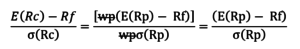
Or E(R_c) = R_f + S_pσ(R_c), where S_p = 

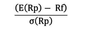
The line E(R_c) = R_f + S_pσ(R_c) is the capital allocation line (CAL). The slope of the line, S_p, is called the Sharpe ratio, or reward-to-risk ratio. The Sharpe ratio measures the increase in expected return per unit of additional standard deviation.

Optimal portfolio

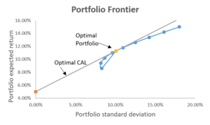
The optimal portfolio consists of a risk-free asset and an optimal risky asset portfolio. The optimal risky asset portfolio is at the point where the CAL is tangent to the efficient frontier. This portfolio is optimal because the slope of CAL is the highest, which means we achieve the highest returns per additional unit of risk. The graph below illustrates this:

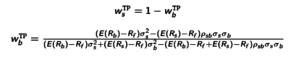
The tangent portfolio weights are calculated as follows:

Summary of capital allocation line

Investors use both the efficient frontier and the CAL to achieve different combinations of risk and return based on what they desire. The optimal risky portfolio is found at the point where the CAL is tangent to the efficient frontier. This asset weight combination gives the best risk-to-reward ratio, as it has the highest slope for CAL.

Download the Free Template

Enter your name and email in the form below and download the free template now!

Additional Resources

Thank you for reading CFI’s guide on Capital Allocation Line (CAL) and Optimal Portfolio. To advance your career, these additional resources will be helpful:

• Portfolio Management Career Profile
• Market Risk Premium
• Sharpe rRatio Definition
• Sharpe Ratio Calculator
• See all capital markets resources
• See all wealth management resources