Equilibrium Term Structure Models

What are Equilibrium Term Structure Models?

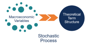
Equilibrium Term Structure Models (also known as Affine Term Structure Models) are stochastic interest rate models used to estimate the correct theoretical term structure. Equilibrium term structure models estimate the stochastic process that describes the dynamics of the yield curve (term structure).

The models identify mis-pricing in the bond market since the estimated term structure is almost never equal to the actual market term structure. They primarily look at macroeconomic variables when estimating the stochastic process that can explain variations in the short-term interest rate.

One-Factor Models vs. Multi-Factor Models

1. One-Factor Models

One-factor models work under the assumption that there is only one unique macroeconomic variable that affects the term structure of interest rates. Although unrealistic, one-factor models provide good approximations of the term structure if the various factors affecting interest rates are highly correlated.

2. Multi-Factor Models

Multi-factor models work under the assumption that there are multiple macroeconomic variables that affect the term structure of interest rates. The accuracy of multi-factor models increases as they incorporate more factors. Such models are usually very complex and require numerical optimization techniques to solve.

Interest Rate Processes

An interest rate process is a general stochastic differential equation of the form:

Where:

• dr is the change in interest rate
• h(r) is the drift rate, which is a general function of the current interest rate
• dt is the change in time
• ϭ(r) is the standard deviation of the current interest rate
• dW is the change in the Weiner Process

The first component on the right-hand side is known as the drift component and the second component on the right-hand side is known as the volatility component. Different equilibrium models model the components differently.

1. Normal Process (or the Gaussian Process)

Changes in forward interest rates (relative to the spot rate) are normally distributed. The rate of change of forward interest rates (i.e., the volatility of forward interest rates) is an increasing function of time and is independent of the current interest rate. For example, the volatility in the 5-year forward interest rate is typically equal to or less than the volatility in the 10-year forward interest rate.

In addition, the volatility in the 5-year forward interest rate and that of the 10-year forward interest rate are independent of the current interest rate. An example of an interest rate model that uses the normal process is the Vasicek Model [d_r = (r₀ – r)hdt + ϭdW].

The Vasicek Model is a one-factor mean reversion model where the short-term interest rate converges to a steady state value, r₀. This model was introduced by Czech mathematician, Oldrich Alfons Vasicek, in his 1977 paper, “An Equilibrium Characterization of the Term Structure.”

2. Squared Normal Process (or the Squared Gaussian Process)

Changes in forward interest rates (relative to the spot rate) are normally distributed. The rate of change of forward interest rates (volatility of forward interest rates) is an increasing function of time and is directly proportional to the square root of the current interest rate. An example of an interest rate model that uses the squared normal process is the Cox-Ingersoll-Ross Model [d_r = (r₀ – r)hdt + ϭ√rdW].

The Cox-Ingersoll-Ross Model (CIR Model) is a one-factor mean reversion model that is a generalization of the Vasicek model. The model was introduced by John Cox, Jonathan Ingersoll, and Stephen Ross, in their 1985 paper, “A Theory of the Term Structure of the Interest Rate,”

3. Log-Normal Process

Changes in forward interest rates (relative to the spot rate) are normally distributed. The rate of change of forward interest rates (volatility of forward interest rates) is an increasing function of time and is directly proportional to the current interest rate. An example of an interest rate model that uses the log-normal process is the Black-Derman-Toy Model [d_r = (r₀ – r)hdt + ϭrdW].

The Black-Derman-Toy Model is a one-factor mean reversion model that was developed by Fischer Black, Emanuel Derman, and Bill Toy.

More Resources

CFI is the official provider of the global Financial Modeling & Valuation Analyst (FMVA)™ certification program, designed to help anyone become a world-class financial analyst. To keep learning and advancing your career, the additional CFI resources below will be useful:

• Central Limit Theorem
• Demand Curve
• Normal Distribution
• Stochastic Oscillator
• See all data science resources