CEILING.PRECISE Function
Rounds up a number to the nearest integer or multiple of significance
What is the CEILING.PRECISE Function?
The CEILING.PRECISE Function[1] is categorized under Excel Math and Trigonometry functions. It will round up a number to the nearest integer or multiple of significance.
As a financial analyst, we can use CEILING.PRECISE in setting the pricing after currency conversion, discounts, etc. When preparing financial models, it helps us round up the numbers per a requirement.
CEILING.PRECISE was introduced in MS Excel 2010 to replace the CEILING function. It was subsequently replaced by the CEILING.MATH function.
Formula
=CEILING.PRECISE(number, [significance])
The CEILING.PRECISE function uses the following arguments:
- Number (required argument) – This is the value which we wish to round off.
- Significance (optional argument) – This specifies the multiple of significance to round the supplied number to.
- If we omit the argument, it takes default value 1. That is, it will round up to the nearest integer. The argument will ignore the arithmetic sign.
- So, remember that, by default, the significance argument is 1.
The CEILING.PRECISE function uses the absolute value of the multiple, so that it returns the mathematical ceiling regardless of the sign of the number and significance.
How to use the CEILING.PRECISE Function in Excel?
To understand the uses of the CEILING.PRECISE function, let’s consider a few examples:
Example 1
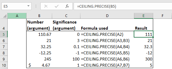
Let’s see the results from the function when we provide the following data:
| Number (argument) | Significance (argument) | Result | Remarks |
|---|---|---|---|
| 110.67 | 111 | As the [significance] argument is omitted, it takes on the default value of 1 and rounds off away from zero. | |
| 21 | 3 | 21 | The function rounds up to the nearest multiple of 3. As 21 is a multiple of 3, we got the result as 21. |
| 32.25 | 0.1 | 32.3 | It rounded up away from 0. |
| -12.25 | -1 | -12 | It rounds -12.25 down (away from 0) to the nearest integer that is a multiple of 1. The arithmetic sign of the [significance] argument is ignored by the function. So, if the value given was 12.25 and significance was -1, the function would be rounded up away from 0. |
| 245 | 100 | 300 | It rounded up to nearest multiple of 100 away from 0. |
| $4.67 | 1 | 5 | It rounded up to nearest multiple of 5 away from 0. |
The formula used and results in MS Excel are shown below:
Example 2
Suppose we wish to know how many cupcakes will fit in a rectangle box of different sizes. We are given the data below:
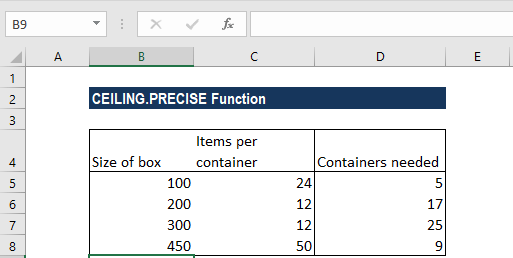
The item per container depicts the number of items, which is the cupcakes to be held in the rectangular box.
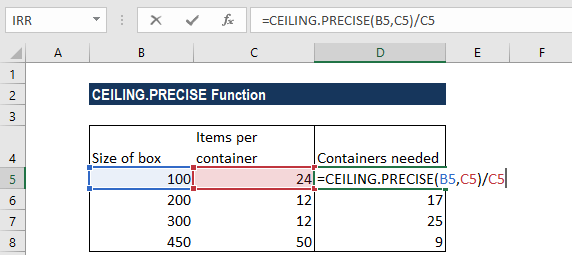
The formula we will use is =CEILING.PRECISE(A2,B2). It rounds up A2 to the nearest multiple of B2 (that is, items per box). The value derived will be divided by the number of containers. For example, in the second row, 100 will be rounded to a multiple of 24 and the result will be divided by 24.
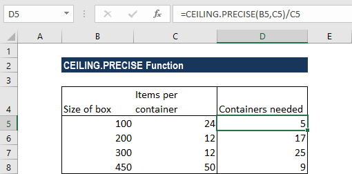
We get the result below:
A few notes about the CEILING.PRECISE Function
- #VALUE! error – Occurs when any of the arguments is non-numeric.
- Instead of the CEILING.PRECISE function, we can use the INT function or CEILING.MATH function.
- The function should be used only for backward compatibility.
Click here to download the sample Excel file
Additional Resources
Thanks for reading CFI’s guide to important Excel functions! By taking the time to learn and master these functions, you’ll significantly speed up your financial analysis. To learn more, check out these additional CFI resources:
- Excel Functions for Finance
- Excel Shortcuts for PC and Mac
- CEILING Function
- CEILING.MATH Function
- CRITBINOM Function
- See all Excel resources
Article Sources
Excel Tutorial
To master the art of Excel, check out CFI’s Excel Crash Course, which teaches you how to become an Excel power user. Learn the most important formulas, functions, and shortcuts to become confident in your financial analysis.

Launch CFI’s Excel Crash Course now to take your career to the next level and move up the ladder!


