CEILING Function

What is the Excel CEILING Function?

The Excel CEILING function[1] is categorized under Math and Trigonometry functions. The function will return a number that is rounded up to a supplied number that is away from zero to the nearest multiple of a given number. MS Excel 2016 handles both positive and negative arguments.

The function is very useful in financial analysis as it helps in setting the price after currency conversion, discounts, etc. When preparing financial models, CEILING helps us round up the numbers as per the requirement. For example, if we provide =CEILING(10,5), the function will round off to the nearest 5 dollars.

Formula

=CEILING(number, significance)

The function uses the following arguments:

1. Number (required argument) – This is the value that we wish to round off.
2. Significance (required argument) – This is the multiple that we wish to round up to. It would use the same arithmetic sign (positive or negative) as per the provided number argument.

How to use the CEILING Function in Excel

To understand the uses of the CEILING function, let’s consider a few examples:

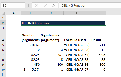
Example 1 – Excel Ceiling

Let’s see the results from using the function when we provide the following data:

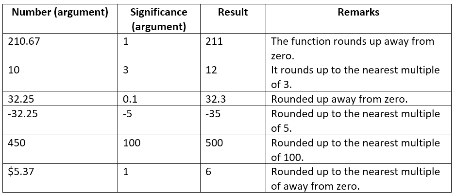
The formula used and results in Excel are shown in the screenshot below:

Example 2 – Using CEILING with other functions

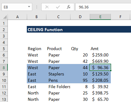
We can use CEILING to highlight rows in a group of data. We will use a combination of ROW, CEILING, and ISEVEN functions. Suppose we are given the data below:

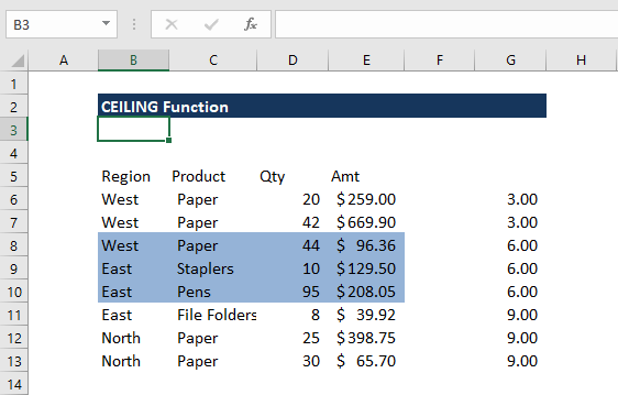
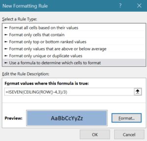
If we wish to highlight rows in groups of 3, we can use the formula =ISEVEN(CEILING(ROW()-4,3)/3) in conditional formatting.

We will get the result below:

In applying the function, remember to select the data before clicking on conditional formatting.

First, we “normalized” the row numbers to begin with 1, using the ROW function and an offset. Here 3 is n (the number of rows to group) and 4 is an offset to normalize the first row to 1 as the first row of data is in row 6. The CEILING function rounds incoming values up to a given multiple of n. Essentially, the CEILING function counts by a given multiple of n.

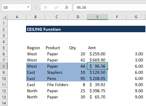
The count shown above in column G is then divided by n, that is in this case =3. Lastly, the ISEVEN function is used to force a TRUE result for all even row groups, which triggers the conditional formatting.

Notes about the Excel CEILING Function

1. #NUM! error – Occurs when:
   • If we are using MS Excel 2007 or earlier versions, provide the significance argument with a different arithmetic sign from the given number argument.
   • If we are using MS Excel 2010 or 2013, if the given number is positive and the supplied significance is negative.
2. #DIV/0! error – Occurs when the significance argument provided is 0.
3. #VALUE! error – Occurs when any of the arguments is non-numeric.
4. CEILING is like MROUND but it always rounds up away from zero.

Click here to download the sample Excel file

Additional Resources

Thanks for reading CFI’s guide to important Excel functions! By taking the time to learn and master these functions, you’ll significantly speed up your financial analysis. To learn more, check out these additional CFI resources:

• Excel Functions for Finance
• Advanced Excel Formulas You Must Know
• CEILING.PRECISE Function
• PRICEDISC Function
• See all Excel resources