COUPDAYSNC Function
Calculates the number of days from the settlement date to the next coupon rate
What is the COUPDAYSNC Function?
The COUPDAYSNC Function[1] is categorized under Excel Financial functions. It helps calculate the number of days from the settlement date to the next coupon rate.
As we are aware, coupon bonds pay interest at regular intervals. MS Excel introduced the COUPDAYSYNC function to calculate the days before we get paid. Thus, it allows us to manage cash flows in an efficient manner.
Formula
=COUPDAYSNC(settlement, maturity, frequency, [basis])
The COUPDAYSNC function uses the following arguments:
- Settlement (required argument) – This is the settlement date of a given security. It is the date after the security is traded to the buyer.
- Maturity (required argument) – This is the date when the security expires.
- Frequency (required argument) – The number of coupon payments per year. The argument can take a value of 1 (annual payment), 2 (semi-annual payments), or 4 (quarterly payments).
- Basis (optional argument) – This specifies the day count basis to be used. It uses one of the following values:
| Basis | Day Count basis |
|---|---|
| 0 or omitted | US(NASD) 30/360 |
| 1 | Actual/actual |
| 2 | Actual/360 |
| 3 | Actual/365 |
| 4 | European 30/360 |
The function will default to zero when omitted. It indicates that the days in the month are counted using the US 30-day method with a 360-day year. When we enter 1 as the basis, the function uses the actual number of days in the month and year. Whereas, when we enter 2, it will count the actual days in the month with a 360-day year, while 3 will assume a 365-day year. When we enter 4 as the basis, it is the same as 1 except that it uses the European 30-day method.
How to use the COUPDAYSNC Function in Excel?
To understand the uses of the COUPDAYSNC function, let’s consider a few examples:
Example 1
Let’s see how the function works when we are given the following data:
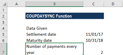
Additionally, we are told that count basis would be 1.
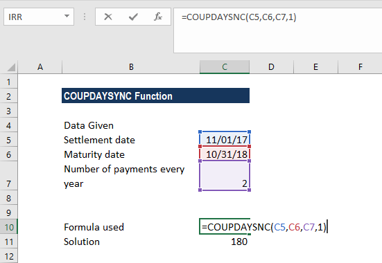
Using the formula =COUPDAYSNC(C5,C6,C7,1), we get 180 as the result. We left the basis as 1 so the function used the Actual/actual as count days.
Example 2
As the function doesn’t accept dates in text format, we need to convert them into a DATE format. Let’s see an example to understand it. Suppose we are given the following data:
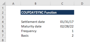
As we need to find the number of days using the function, so we need to first convert the dates given in text format.
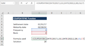
The formula to be used would be =COUPDAYS(DATE(2017,1,31),DATE(2022,2,28),1,2).
The result we get here is 28. Excel first converted the dates in text format into proper dates and then calculated the number of days. Here we used 1 as the frequency and 2 as the basis.
Few notes about the COUPDAYSNC Function:
- #NUM! error – Occurs in the following scenarios:
- When the settlement date provided is greater than or equal to (≥) the maturity date.
- When the given frequency argument provided by the user is not equal to 1, 2, or 4.
- When the given basis argument is a number other than 0, 1, 2, 3, or 4.
- #VALUE! error – Occurs in the following scenarios:
- When the given settlement date or the maturity date is not a valid date. Remember that we need to enter dates in date format or else use the DATE function to convert them to proper dates. The function doesn’t work when dates given are in text format. For example, =COUPDAYSNC(“1/25/2023″,”11/15/2024”,2,1) = #VALUE.
- Any of the arguments given is non-numeric.
- The COUPDAYSNC function truncates all arguments to Integers.
Click here to download the sample Excel file
Additional Resources
Thanks for reading CFI’s guide to the Excel COUPDAYSNC function. By taking the time to learn and master these functions, you’ll significantly speed up your financial analysis. To learn more, check out these additional CFI resources:
- Excel Functions for Finance
- Advanced Excel Formulas Course
- COUPNUM Function
- COUPDAYBS Function
- See all Excel resources
Article Sources
Excel Tutorial
To master the art of Excel, check out CFI’s Excel Crash Course, which teaches you how to become an Excel power user. Learn the most important formulas, functions, and shortcuts to become confident in your financial analysis.

Launch CFI’s Excel Crash Course now to take your career to the next level and move up the ladder!


