COUPDAYBS Function
Calculates the number of days from the start of a coupon’s period until the settlement date
Key Highlights
- The COUPDAYBS is one of the financial functions in Microsoft that calculates the number of days between the settlement date and the last coupon payment date.
- Using the settlement date, maturity date, the frequency of coupon payments and the day count basis, a financial analyst can easily calculate the amount of accrued interest by multiplying the output by the coupon rate.
What Does the COUPDAYBS Function Do?
The COUPDAYBS Function[1] is a financial function in Microsoft Excel that calculates the number of days from the beginning of a coupon period until its settlement date. In other words, the COUPDAYBS function helps return the number of days between the settlement date and the last time a coupon was paid.
In the capital markets, we call this coupon period between the previous coupon payment date and the settlement date accrued interest. In other words, if two parties were to transact on a bond, the COUPDAYBS function can be used to find the number of days’ interest that the buyer of the bond needs to pay to the seller of the bond upon settlement date.
Accrued Interest Payments
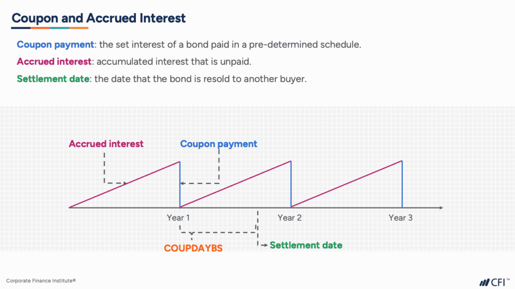
If we look at the following figure, we have a simplified diagram depicting the interest cashflows from a three-year bond that pays coupons once a year by the bond issuer to the bondholder, called an annual-pay bond. The accrued interest is the amount of interest due to the holder of the bond and is paid at the end of every year at the coupon payment date, shown in blue.
Usage Scenarios for the COUPDAYBS Function
1. Secondary market transactions
Let’s imagine a situation where a bondholder decides to sell the bond to another investor in the secondary market before the maturity date, somewhere between the end of the first and second years.
If we illustrate that point in time as the settlement date (in green above), you can see that the interest for year two of the bond is yet to be paid by the issuer. However, the new buyer of the bond needs to compensate the seller for the bond interest that they should be owed for holding the bond from the last coupon payment date to the settlement date.
The number of days from the beginning of the latest coupon payment date period to the settlement date is what the Excel COUPDAYBS function easily calculates (shown in orange above).
The function returns the number of days, which then can be used by financial analysts to calculate the amount of accrued interest that is owed by the buyer of the bond to the seller by multiplying the number of days by the coupon rate.
2. Bond issuer calculations
Next, let’s consider a situation where a bond issuer needs to figure out how much interest they need to pay at the next coupon date. They could use a calendar to count the number of days from the previous coupon date to the next coupon date.
However, they might consider the day count basis for their bond, as well as the frequency of coupon payments per year.
By using the COUPDAYBS function, they can easily calculate the number of days from the beginning of the coupon period to the next coupon date by setting the settlement date as the next coupon payment date, as we see in the diagram below.
Again, by using the number of days that the COUPDAYBS function returns, a financial analyst can calculate the amount of interest to be paid by multiplying the number of days by the coupon rate.

COUPDAYBS Syntax
=COUPDAYBS(settlement, maturity, frequency, [basis])
The COUPDAYSBS function uses the following arguments:
- Settlement (required argument) – This is the settlement date of a given security. It is the date after the security is traded to the buyer.
- Maturity (required argument) – This is the date when the security expires.
- Frequency (required argument) – This is the number of coupon payments per year. The argument can take a value of 1 (annual payment), 2 (semi-annual payments), or 4 (quarterly payments).
- Basis (optional argument) – It specifies the day count basis to be used. It uses one of the following values:
| Basis | Day Count basis |
|---|---|
| 0 or omitted | US(NASD) 30/360 |
| 1 | Actual/actual |
| 2 | Actual/360 |
| 3 | Actual/365 |
| 4 | European 30/360 |
The function will default to zero when omitted. It indicates that the days in the month are counted using the US 30-day method with a 360-day year. When we enter 1 as the basis, the function uses the actual number of days in the month and year.
Whereas, when we enter 2, it will count the actual days in the month with a 360-day year, while 3 will assume a 365-day year. When we enter 4 as the basis, it is the same as 1, except that it uses the European 30-day method.
How to Use the COUPDAYBS Function in Excel?
To understand the uses of the COUPDAYBS function, let’s consider a few examples:
Example 1
Let’s see how the function works when we are given the following data:
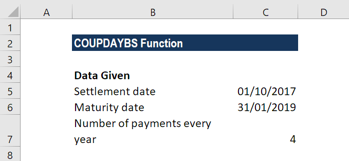
Additionally, we are told that 4 payments are made per year.
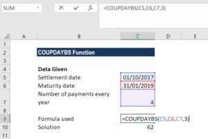
Using the formula =COUPDAYBS(C5,C6,C7,3), we get the result 62 as the result. We used the Actual/365 as count days.
Example 2
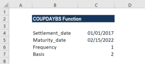
As the COUPDAYBS function doesn’t accept dates in text format, we need to convert them into DATE format. Let’s see an example to understand it. Suppose we are given the following data:
As we need to find the number of days using the function, we need to first convert the dates given into text format.
The formula to be used would be =COUPDAYBS(DATE(2017,1,1),DATE(2022,2,15),1,2).
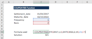
The result we get here is 321. Excel first converted the dates into text format into proper dates and then calculated the number of days. Here, we used 1 as the frequency and 2 as the basis.
Few Notes About the COUPDAYBS Function
- #NUM! error – Occurs in the following scenarios:
- When the settlement date is greater than or equal to (≥) the maturity date.
- When the frequency argument provided by the user is not equal to 1, 2 or 4.
- When the given basis argument is a number other than 0, 1, 2, 3 or 4.
- #VALUE! error – Occurs in the following scenarios:
- When the given settlement date or the maturity date is not a valid date. Remember that we need to enter dates in date format or else use the DATE function to convert them into proper dates. The function doesn’t work when the dates given are in text format. For example, =COUPDAYBS(“1/25/2023″,”11/15/2024”,2,1) = #VALUE
- Any of the arguments given is non-numeric.
- The COUPDAYBS function truncates all arguments to Integers.
Click here to download the sample Excel file
Additional Resources
Thanks for reading CFI’s guide to the COUPDAYBS Excel function. By taking the time to learn and master Excel functions, you’ll significantly speed up your financial analysis. To learn more, check out these additional CFI resources:
Excel Tutorial
To master the art of Excel, check out CFI’s Excel Crash Course, which teaches you how to become an Excel power user. Learn the most important formulas, functions, and shortcuts to become confident in your financial analysis.

Launch CFI’s Excel Crash Course now to take your career to the next level and move up the ladder!


