COVAR Function

What is the COVAR Function?

The COVAR Function[1] is categorized under Excel Statistical functions. It will calculate the covariance of two sets of values.

As a financial analyst, suppose we want to see how two stocks may move together in the future. Looking at their historical prices, we can determine if the prices tend to move with each other or opposite each other. It allows us to predict the potential price movement of a two-stock portfolio.

A high, positive covariance value between two stocks implies that when the price of one goes up, that of the other usually does, too.

A high negative figure or value means that when one stock advances, the other generally retreats. If the figure is close to zero, with either a positive or negative sign, the two stocks act mostly independently.

Covariance Formula

=COVAR(array1, array2)

The COVAR function uses the following arguments:

1. Array1 (required argument) – This is a range or array of integer values.
2. Array2 (required argument) – Another range or array of integer values.

Notes

• If the given arrays contain text or logical values, they are ignored by the COVAR function.
• The data should contain numbers, names, arrays, or references that are numeric. If some cells do not contain numeric data, they are ignored.
• The data sets should be of the same size, with the same number of data points.
• The data sets should neither be empty, nor should the standard deviation of their values equal zero.

How to use the COVAR Function in Excel?

As a worksheet function, the COVAR function can be entered as part of a formula in a cell of a worksheet. To understand the uses of the function, let’s consider an example:

Example

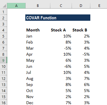
Suppose we are given the following data:

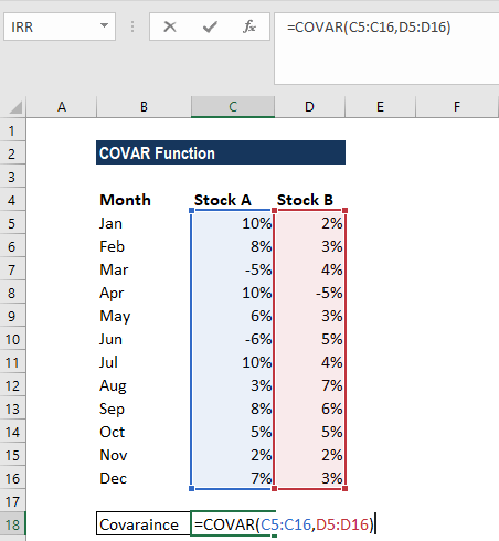
We wish to find out covariance. The covariance of the values in columns B and C of the spreadsheet can be calculated using the COVAR function using the formula =COVAR(B2:B13, C2:C13).

We get the results below:

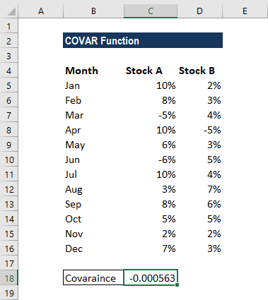
It gives the result -0.000563, which indicates a negative correlation between the two sets of stocks.

A few pointers about the COVAR Function:

1. The function was introduced in MS Excel 2000.
2. #VALUE! error – Occurs when one or both of the supplied data arrays are empty.
3. #N/A! error – Occurs if the given arrays are of different lengths.
4. In MS Excel 2010, the COVAR function was replaced by the COVARIANCE.P function. However, COVAR is still available in MS Excel 2010 (stored in the list of compatibility functions) to allow compatibility with earlier versions of Excel.

Click here to download the sample Excel file

Additional Resources

Thanks for reading CFI’s guide to the Excel COVAR function. By taking the time to learn and master these functions, you’ll significantly speed up your financial analysis. To learn more, check out these additional CFI resources:

• Excel Functions for Finance
• Advanced Excel Formulas You Must Know
• Financial Modeling Certification Program
• COVARIANCE.S Function
• See all Excel resources