Excel ROUNDDOWN
How to round a number down in Excel
What is the Excel ROUNDDOWN Function?
When performing financial analysis in Excel, it’s often useful to round down a number to either a decimal place or a whole number. Thankfully, with the Excel ROUNDDOWN Function,[1] this task is quite easy, even for a large dataset.
In this tutorial, we will show you how to round a number down in Excel using the =ROUNDDOWN() function.
This function will save you time when building a financial model and improve your accuracy in Excel.
How the Excel ROUNDDOWN function works
The ROUNDDOWN function in Excel requires you to reference a number and then specify how many units (decimal places) you want to round it to.
=ROUNDDOWN()
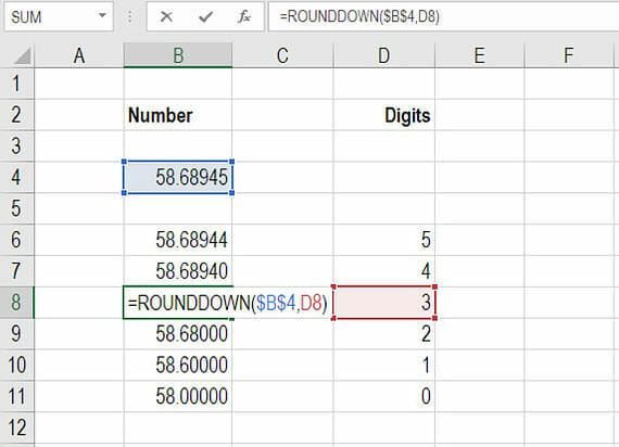
In the example below, we have shown you how to create a table that uses the formula to link to one number and then return a certain number of decimal places.
Step 1: type “=ROUNDDOWN(“
Step 2: link to the cell you want to round down and add a comma
Step 3: type the number of units, or link to a cell that contains the number of units you want to display
Step 4: close bracket and press enter.
In the screenshot below you will see an example of the Excel round down function in action.
Click here to download the Excel template.
More Relevant Excel Resources
Thank you for reading CFI’s guide to the Excel ROUNDDOWN function. Excel is an important part of any financial analyst’s job and critical for performing world-class financial analysis. CFI’s mission is to help you along your path and advance your career as quickly as possible by giving you the tools and training you need to perform great financial analysis.
To become an Excel power user please check out our Excel Resources to learn all the most important functions, formulas, shortcuts, tips, and tricks.
Article Sources
Excel Tutorial
To master the art of Excel, check out CFI’s Excel Crash Course, which teaches you how to become an Excel power user. Learn the most important formulas, functions, and shortcuts to become confident in your financial analysis.

Launch CFI’s Excel Crash Course now to take your career to the next level and move up the ladder!


