How to Find and Remove Duplicates in Excel

Duplicate Values in Excel

Microsoft Excel is one of the most commonly used data analysis tools in the world. Because of this, Excel is often used with ERP systems or general ledgers to analyze various data sets. However, it’s sometimes possible for data to become duplicated. Duplicate data is almost always a mistake, which can ultimately taint any analysis.

Depending on the size of the data, finding duplicates in Excel may be quite difficult and time consuming. A key skill that analysts must master is the ability to remove duplicate data in an Excel worksheet. Fortunately, there are various ways to find duplicates in Excel, and remove them if necessary.

How to Find Duplicates in Excel

There are several different ways to find and remove duplicates in Excel. Let’s take a look at some of them.

1. Find Duplicates in Excel Using Conditional Formatting

Excel’s Conditional Formatting tool is probably the quickest and easiest way to find duplicate records. With a couple of keystrokes (or mouse clicks), Conditional Formatting will quickly highlight duplicates.

First, select the data that may contain duplicates. To access Conditional Formatting, go to the Home ribbon in Excel and select Conditional Formatting. From there, select Highlight Cells Rules and then select Duplicate Values, as shown in the screenshot below. You can apply your own formatting style or use one of Excel’s pre-formatted highlights.

Alternatively, you can also select unique values instead of duplicates, depending on your preference.

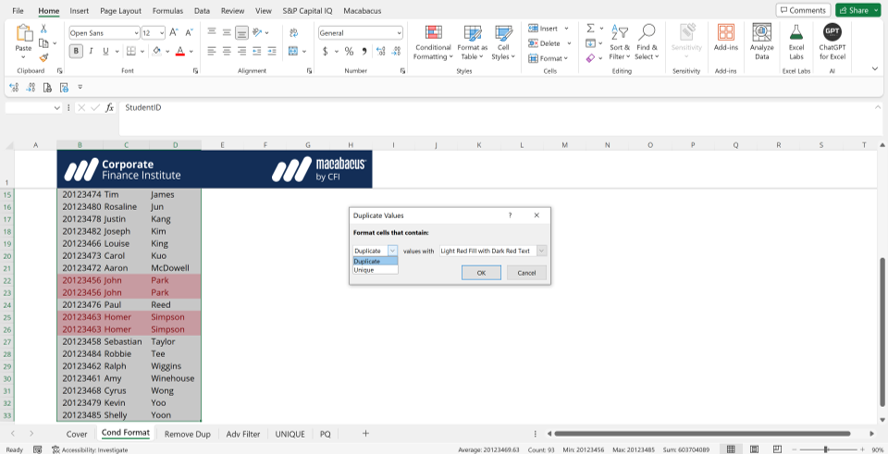
You can see in our sample file that duplicates have been highlighted with a light red fill color and dark red text.

You can also remove the Conditional Formatting by selecting Home -> Conditional Formatting -> Clear Rules.

Download Free Template

Download the free Find and Remove Duplicates in Excel Template now to advance your knowledge.

2. Remove Duplicates Feature in Excel

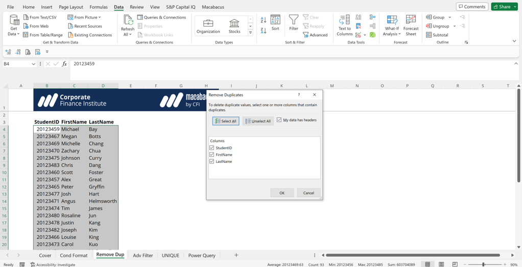
Excel also has an easy-to-use, built-in feature known as Remove Duplicates.

To remove duplicates, first select the appropriate data. To access the Remove Duplicates feature, go to the Data tab on the Excel ribbon. The Remove Duplicates button is small but is highlighted in the orange square box in the screenshot below. Alternatively, you can access Remove Duplicates using the shortcut keys Alt+A+M.

A dialog box will then pop up. If your data has actual column headers, you can select the option “My data has headers,” otherwise, Excel will take a “guess” at the headers. From there, you can select the columns with duplicate data.

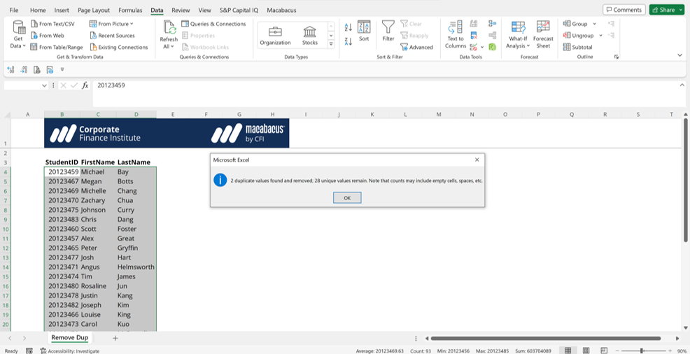
After pressing enter, Excel will remove the duplicate values.

3. Using Advanced Filter for Unique Values

The Filter tool in Excel can be used in multiple different ways, including filtering by text or numbers. What many Excel users don’t realize is that there is advanced functionality that filters out duplicate values.

To use Advanced Filter, select the data you want to filter and go to Data on the Excel ribbon. Then select Advanced, as shown in the screenshot below.t35dwx

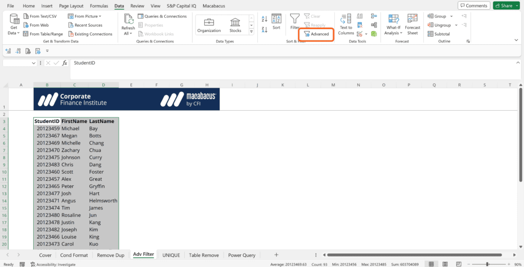
From there, a dialog box will pop up. You can filter the list in place or copy it to another location. But the key here is to select “Unique records only.”

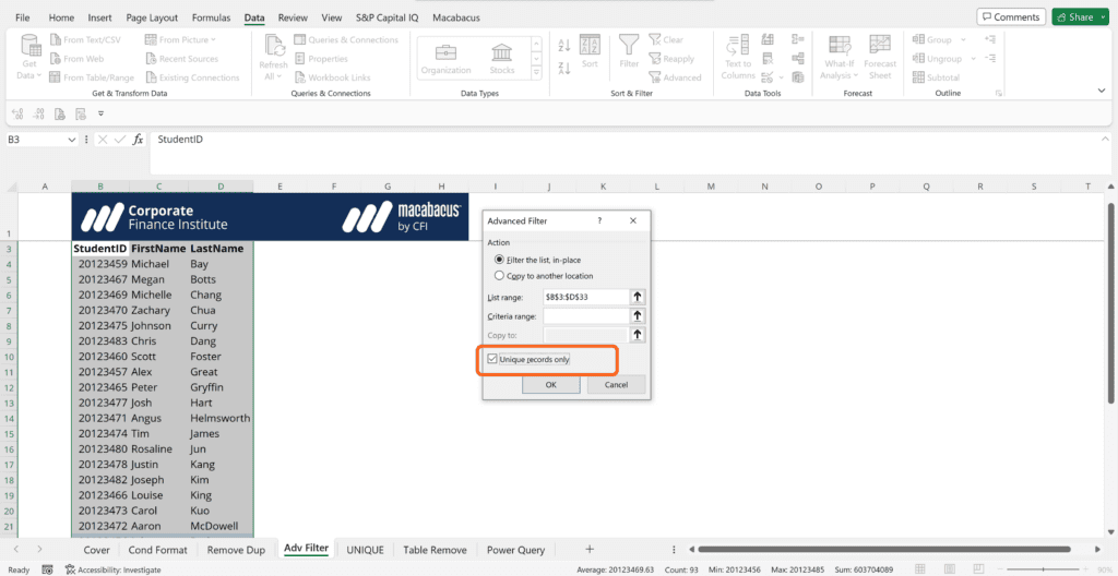
From there, you will have a list of unique data that you can manipulate as necessary.

4. Remove Duplicates Using the UNIQUE Function

One of the disadvantages to the previous techniques is that if you add data, you will then have to make sure 1) the Conditional Formatting range is updated, 2) re-run the Remove Duplicate tool, or 3) re-filter for unique records.

Fortunately, Microsoft recently added the UNIQUE function to some versions of Excel. The UNIQUE function returns a list of unique values in a list or range and is very easy to use.

Simply type =UNIQUE in one cell and select the range of data you want to extract unique values from. Excel will automatically fill in the results of the UNIQUE function beneath the cell you entered the function in.

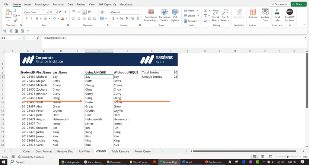
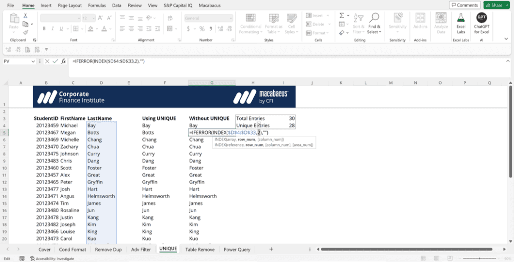
Notice the light blue outline the two orange arrows are pointing to in the screenshot above. The UNIQUE function is what is known as a dynamic array formula. Dynamic array formulas can return arrays of variable size. These formulas create what is called “spilling” in that the formula is automatically and dynamically copied down to capture the appropriate data. In this case, the UNIQUE function pulls out all unique last names and spills the formula down 28 rows (there are 28 unique last names and 30 total entries, as shown in the screenshot above).

If UNIQUE is unavailable in your version of Excel, you can create a long, complex formula that should still work. For example, the formula in cell G4 below will still extract unique last names. Let’s break down this long formula into easier-to-understand steps.

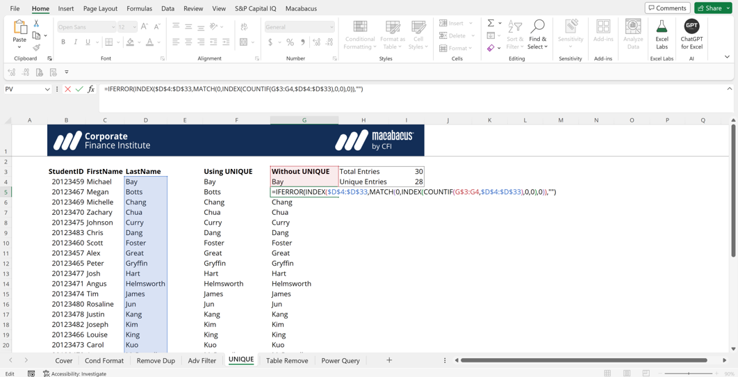
Here is the formula in cell G5: =IFERROR(INDEX($D$4:$D$33,MATCH(0,INDEX(COUNTIF(G$3:G4,$D$4:$D$33),0,0),0)),””).

So what exactly is this formula doing?

COUNTIF counts the number of times something occurs according to a specific criterion. The first argument in COUNTIF is the range of data that needs to be counted. The second argument is the criterion. In this case, COUNTIF is looking at the range of data from G3 to G4 and looking to see if that range contains any of the last names in the range D4 to D33. In this case, since COUNTIF is looking at a range of data (D4 to D33), it returns multiple results in the form of {1;0;0;0;0;0;0;0;0;0;0;0;0;0;0;0;0;0;0;0;0;0;0;0;0;0;0;0;0;0}. Basically, the COUNTIF found the last name “Bay” 1 time in the range D4 to D33 and no other times in that 30-cell data range.

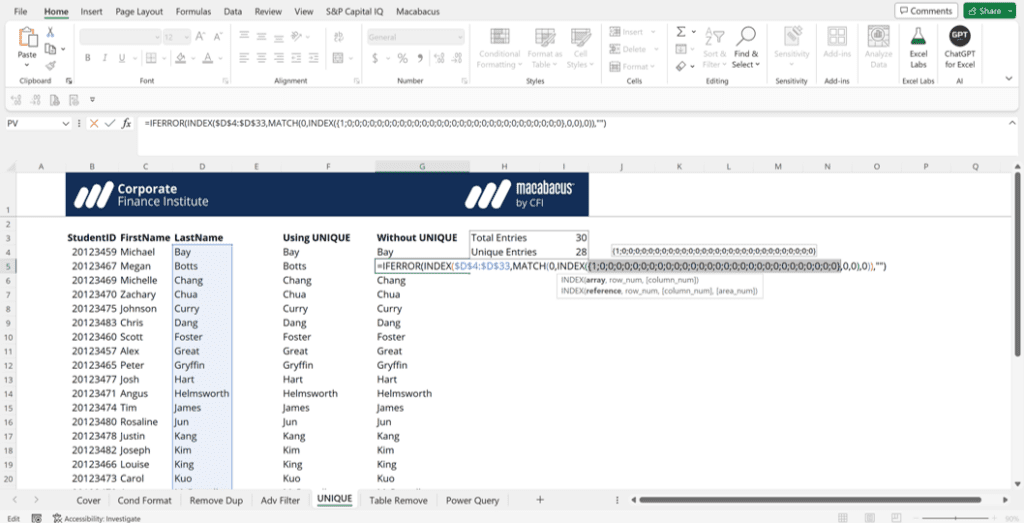
The INDEX function outside of COUNTIF also returns multiple values, which is the same as the COUNTIF: {1;0;0;0;0;0;0;0;0;0;0;0;0;0;0;0;0;0;0;0;0;0;0;0;0;0;0;0;0;0}.

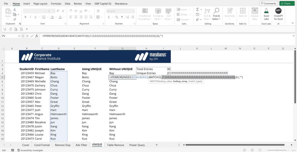
The MATCH function returns the position of a specified value within the array. In this case, MATCH is looking for 0 in the array {1;0;0;0;0;0;0;0;0;0;0;0;0;0;0;0;0;0;0;0;0;0;0;0;0;0;0;0;0;0}. The first time 0 appears in this array is in the second “position,” so the MATCH function returns a 2.

From there, this becomes a classic use of INDEX and MATCH. The “outer” INDEX function uses the range of last name and references the second name, which is “Botts” (since MATCH returned a 2).

The IFERROR function simply returns an empty cell if there is an error with the INDEX/MATCH combination. An empty cell can be created by using two double quotes with no space: “”. A #N/A error is returned when all of the unique names have been captured. Since all of the unique values have been extracted for our list, we are left with a couple of blank cells, as shown in the screenshot below.

5. How to Remove Duplicates in Excel with Power Query

Power Query is an available tool in Excel that can be used to manipulate data and is commonly used for data analysis and business intelligence.

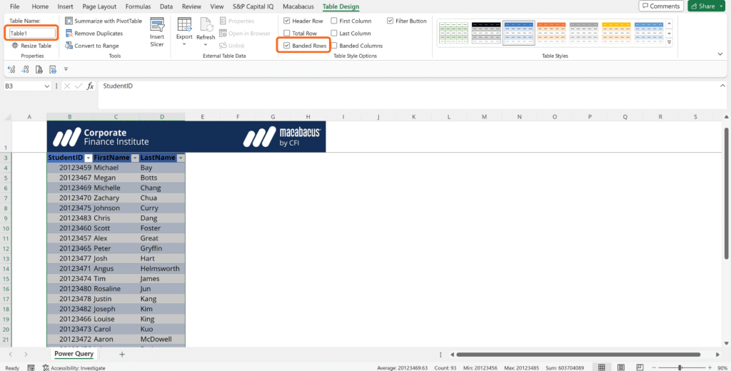
In order to use Power Query for this, we first need to convert our data to an Excel Table. Select the applicable data, then go to Insert on the Excel ribbon and select Table. Alternatively, you can use the shortcut key Ctrl T.

Excel will then confirm the data range and ask if the data has headers. Press OK to create the table.

Excel will then add banded row coloring and filters to the data. The table will also be named (in this case, Table1 since it’s the first table we created).

After the table has been created, go to the Data tab on the Excel ribbon and select From Table/Range. After selecting that, the Power Query Editor will open with the applicable data.

After Power Query Editor opens up, simply select Remove Rows, then Remove Duplicates.

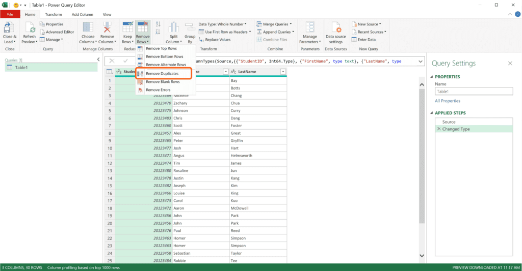
After this, you’ll notice there are now only 28 rows versus the original data, which had 30 rows. Additionally, there is a Removed Duplicates step under Applied Steps in the Power Query Editor.

Related Readings

Thank you for reading CFI’s guide on Finding Duplicates in Excel. To keep learning and developing your knowledge base, please explore the additional relevant resources below:

• Formula vs Function
• Advanced Excel Formulas
• Excel Fundamentals – Quick Start Guide
• Power Query Fundamentals Course
• See all Excel resources