PDURATION Function

What is the PDURATION Function?

The PDURATION Function[1] is an Excel Financial function. It helps the user calculate the time or the specific number of periods required for an investment made to reach a particular value.

In simple terms, it will answer the question: Suppose we invested $1,000,000 at 4% per annum – how long will it take for our investment to reach $1,500,000?

The PDURATION function was introduced in MS Excel 2013 and is unavailable in earlier versions.

Formula

=PDURATION (rate, pv,fv)

The PDURATION function uses the following arguments:

1. Rate (required argument) – This is the interest period per year.
2. Pv (required argument) – The present value of the investment.
3. Fv (required argument) – This is the future value of the investment.

How to use the PDURATION Function in Excel?

To understand the PDURATION function, let’s consider a few examples:

Example 1

Let’s assume that on an initial investment of $1 million, we wish to get $1.5 million when the interest rate is 4% per annum. To see how much time it will take to reach the desired amount, we will use the formula below:

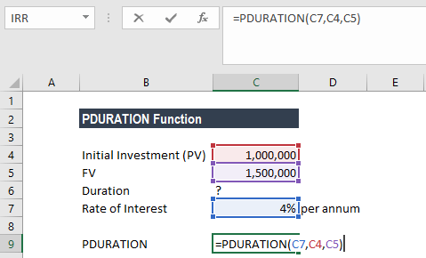
We get the result below:

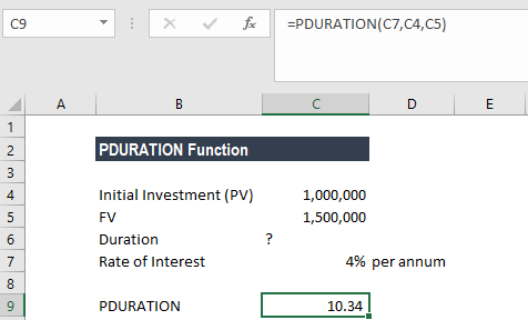
So, it would take 10.34 years for the investment to reach $1.5 million. The PDURATION function is quite helpful in financial planning. With specific financial goals in mind, the function will tell us how much time it will take to achieve the goal with the money on hand.

Example 2

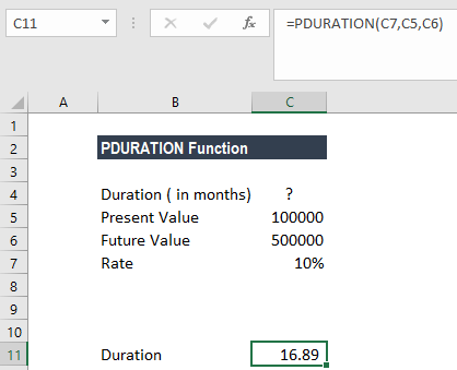
In the example below, let’s assume we are given the rate of interest per period as 10%, the FV, and the PV.

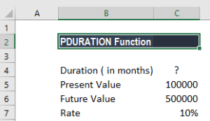
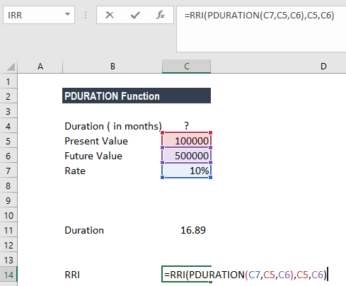
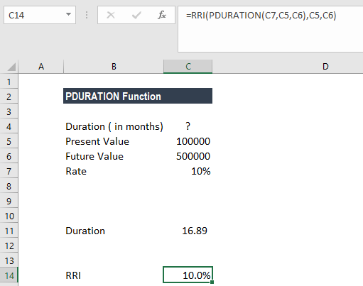
Based on the information, we wish to find out RRI along with duration. We can first find the duration, which is the number of periods that would be required for the investment of $100,000 to reach $500,000. Afterward, we can use the RRI function. The formula would be:

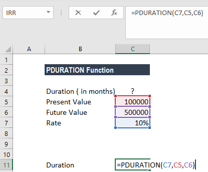
So, in our example, PDURATION says it will take approximately 17 years to get to $500,000.

If we wish to know what would be the CAGR be, we use the RRI function. RRI will tell us that the investment growth rate would be 10%. We can also use the following combined formula to get RRI.

Example 3

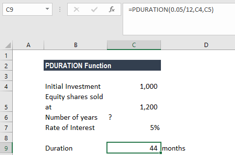
Now let’s take an example wherein we wish to know the number of months and not years. Let’s see how the formula needs to be changed.

In this example, for an initial investment of $1,000 at 5% interest per annum, we need to know how many months it will take to reach $1,200. The formula to use is:

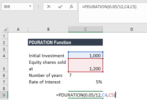
In the formula above, we divided the interest rate with 12 (number of months) to get the result in months.

The result we got is 44 months. The investment will take 44 months to reach $1,200.

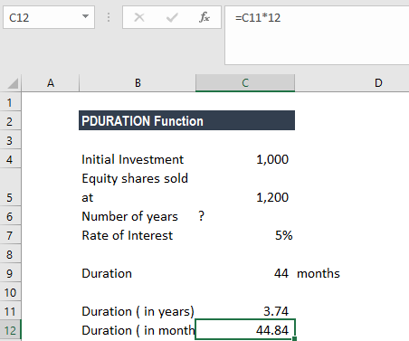
Another way to do it is to get the result in years and then multiply the result by 12 (number of months) to get the result in months, as shown below:

Few pointers about the PDURATION Function 

1. #NUM! error – Occurs in the following situations:
   • When the arguments given are negative or equal to 0.
   • Any of the given arguments of the formula is in an invalid format.

2. #VALUE! error – Occurs when any of the arguments in the formula uses valid data types that are non-numeric.

Click here to download the sample Excel file

Additional Resources

Thanks for reading CFI’s guide to the Excel PDURATION function. By taking the time to learn and master these Excel functions, you’ll significantly speed up your financial analysis. To learn more, check out these additional CFI resources:

• Excel Functions for Finance
• Advanced Excel Formulas You Must Know
• Excel Shortcuts for PC and Mac
• MDURATION Function
• See all Excel resources