ROW Function

How to Alternate Row Color in Excel?

To alternate row color in excel, you can do so by applying conditional formatting, with a combination of functions. The ROW Function[1] is an Excel TEXT function, that will return the first row within a given reference or the number of the current row. If you combine the ROW with the ISODD/ISEVEN and the CEILING function, you can easily alternate the row color of a selected range of cells. 

Depending on your purpose for alternating row colors, there is a simple way to do it. If you select the range that you desire and then insert a table, this should automatically alternate the row colors, there are multiple table styles that you can select from to fit the style guide that you are looking for. This guide is for a little more complicated, but with a greater room for customization, option.

In financial analysis, alternating row color can improve the readability of your spreadsheet. It also facilitates grouping information, such as highlighting alternating groups of n rows.

ROW Function – Step-by-Step Guide

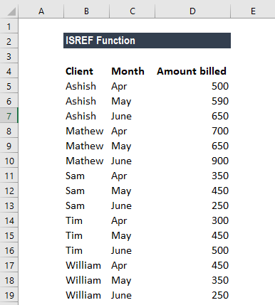
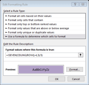
Suppose that we have a table of values in Excel such as the one below. If we want to alternate our row color for every n rows, – i.e., 3 rows grey, 3 rows no fill – you should select the range of rows that you want to apply the alternating rows. Then you should select 

The formula to use would be =ISEVEN(CEILING(ROW()-4,3/3).

We will get the results below:

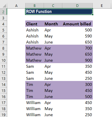
In the formula above, we first “normalize” the row numbers to begin with 1 using the ROW function and an offset.

Here, we used an offset of 4. The result goes into the CEILING function, which rounds incoming values up to a given multiple of n. Essentially, the CEILING function counts by a given multiple of n.

The count is then divided by n to count by groups of n, starting with 1. Finally, the ISEVEN function is used to force a TRUE result for all even row groups, which triggers the conditional formatting.

Odd row groups return FALSE, so no conditional formatting is applied.

We can replace ISEVEN with ISODD to shade rows starting with the first group of n rows, instead of the second.

Click here to download the sample Excel file

The ROW() Function

=ROW(reference)

The ROW function uses Reference as an argument. The reference is supposed to be a cell, so that the function will retrieve the row value.

If you instead leave the argument blank and simply enter =ROW(), the function will return the row of where the function is. So, for example, let’s assume you enter the function =ROW() on cell D22, the function will return 22. If instead, you enter the function =ROW(C7), the function will return the 7.

A reference can not refer to multiple areas.

Additional Resources

Feel free to contact CFI if you have any further questions on how to use the row function and other. By taking the time to learn and master these functions, you’ll significantly speed up your financial modeling. To learn more, check out these additional CFI resources:

• Excel Functions for Finance
• Advanced Excel Formulas Course
• Excel Shortcuts for PC and Mac
• COLUMN Function in Excel
• See all Excel resources