Get Certified for Financial Modeling (FMVA)®
Gain in-demand industry knowledge and hands-on practice that will help you stand out from the competition and become a world-class financial analyst.
Use advanced Excel formulas to perform powerful and dynamic financial analysis
For financial analysts in investment banking, equity research, FP&A, and corporate development, it is advantageous to learn advanced Excel skills because it makes you stand out from your competitors.
In this article, we will go through some of the best industry practices that will help you dramatically speed up financing modeling and perform a powerful and dynamic analysis. This will also help you increase the use of the keyboard over the mouse to save time in financial analysis in the long run. Learn how to create dynamic dates, sums, averages, and scenarios in Excel.
When building financial models, you always start with setting the start and end dates. Instead of inserting the dates manually, you can use the IF statements to make it dynamic.
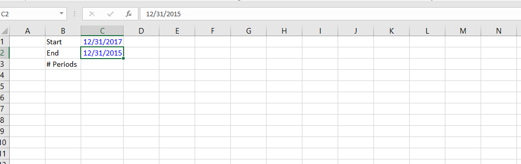
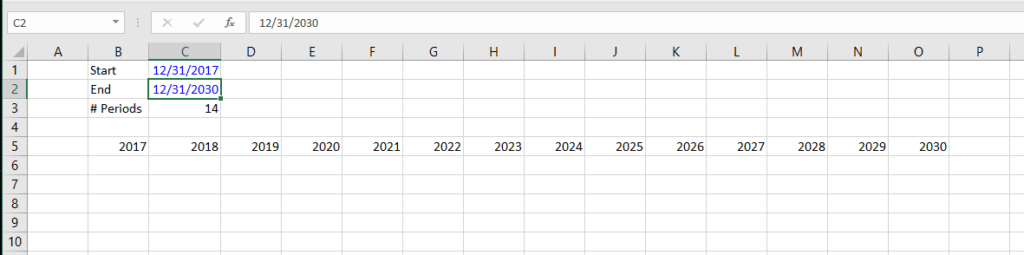
1. Set the start and end date for your model. Change the font to the blue color to show that they are hard-coded numbers.
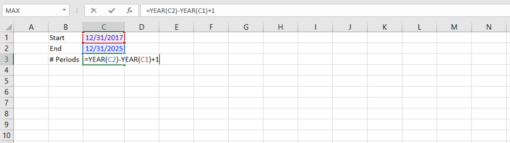
2. Calculate the number of periods using formula =YEAR(C2)-YEAR(C1)+1. You need to add one period because the beginning and ending periods are included in the count.
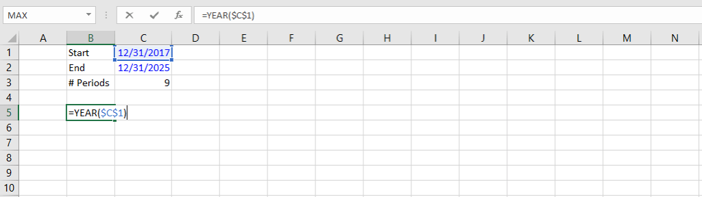
3. Set up the dynamic dates across row 5 using formulas. In cell B5, insert start date =YEAR($C$1). Press F4 to anchor the cell reference.
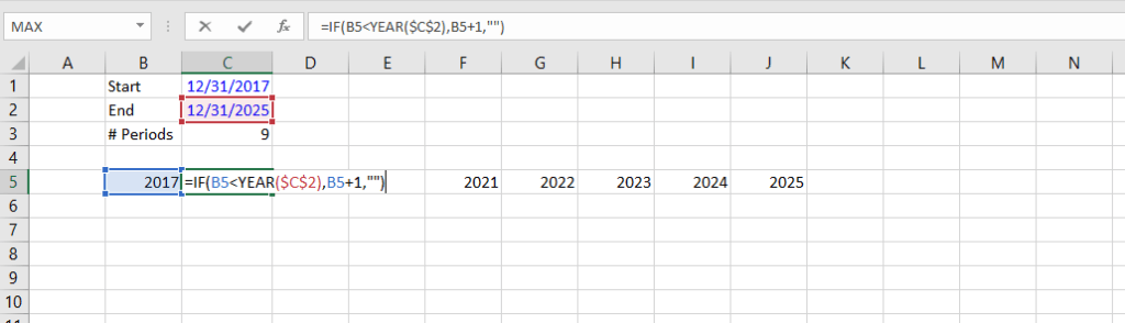
4. In cell B6, type formula =IF(B5<YEAR($C$2),B5+1,””) to insert the dynamic date. Hold SHIFT and right arrow, then press CTRL + R to fill down the cells. It will fill the cells to the right until the end date.
5. You can now easily modify the dates without manually going through each of the cells. For example, if you change the end date to 12/31/2030, the cells will automatically fill to the right until it reaches 2030.
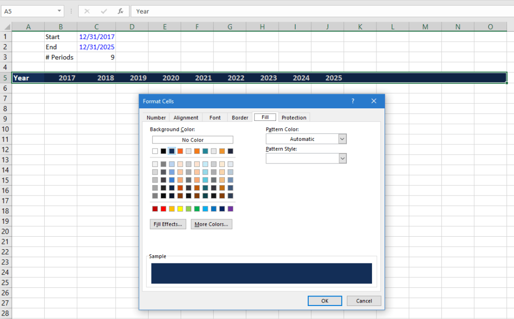
6. Press SHIFT + CTRL + right arrow to select the entire date section and press CTRL + 1 to open up the Format Cells window. Change the fill to dark blue and font to white color, then press OK. Press CTRL + B to bold font and increase the size to 12. You now have a header where all your financial analysis flows below.
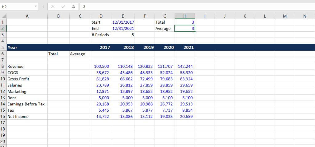
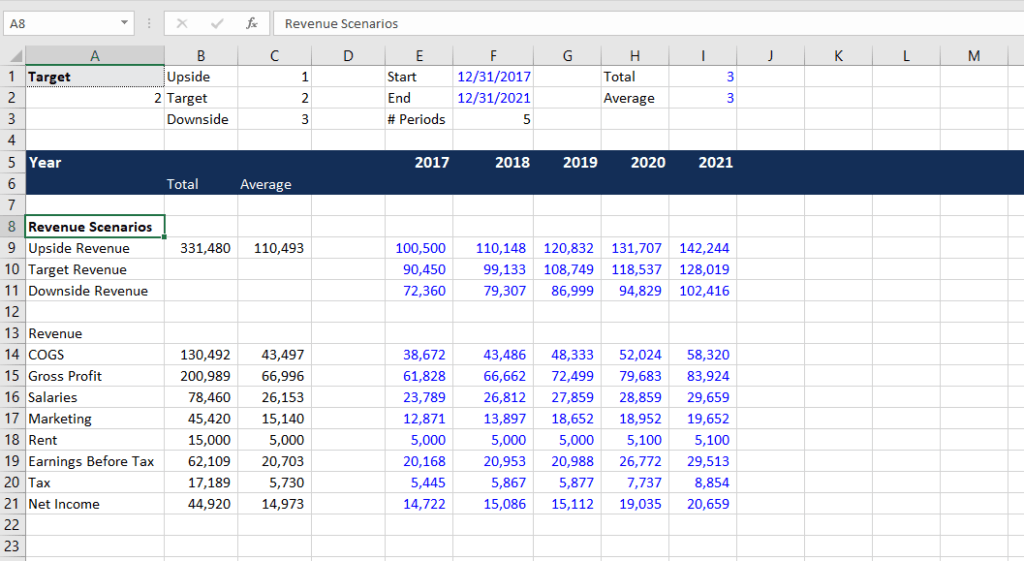
We will now input some data and start building the model. You can copy data from financial statements and paste the value by pressing ALT + E + S and V for values. Use ALT + H + F + C to change the font to blue color. In this set of data, the start year is 2017 and the end year is 2021.
7. Press ALT + I + C twice to insert two columns to the left of 2017 data. We will use them as total and average columns. At the top, insert Total and Average in cell G1 and G2, and put 3 beside both cells. These are the number of periods we would like to include in the calculations. For models with longer periods of historic data, you may want to use only a few periods to calculate your total and average.
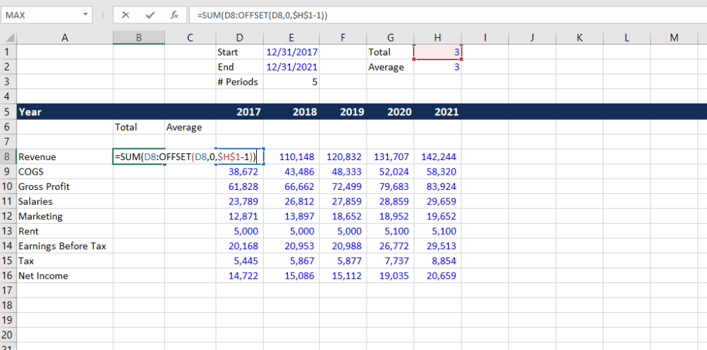
8. Now we’ll use the OFFSET function to set up the total column. In cell B8, type =SUM(D8:OFFSET(D8,0,$H$1-1)). The OFFSET function allows us to select a range of data with reference to the amount of periods we would like to include which we input in cell H1.
We need to subtract 1 from the number of columns because we only want to include two more columns (i.e., column D to F). You can change the hard-coded number of total periods to change the total value.
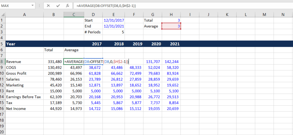
9. The formula for the average is similar, except the cell reference used in the number of periods is H2: =AVERAGE(D8:OFFSET(D8,0,$H$2-1)). Press SHFIT + down arrow and CTRL + D to fill down the cells.
Next, we will set up some scenarios. In cell B1 to B3, set three scenario names: upside, target, and downside cases.
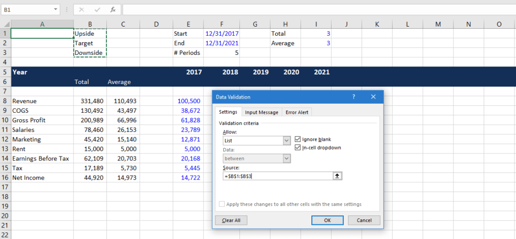
10. In cell A1, press ALT + A + V + V (A for Data, V for Data Validation, and V for Validation). We will create a drop-down list for the scenarios. Choose List and select cell B1 to B3 as the source. Press OK.
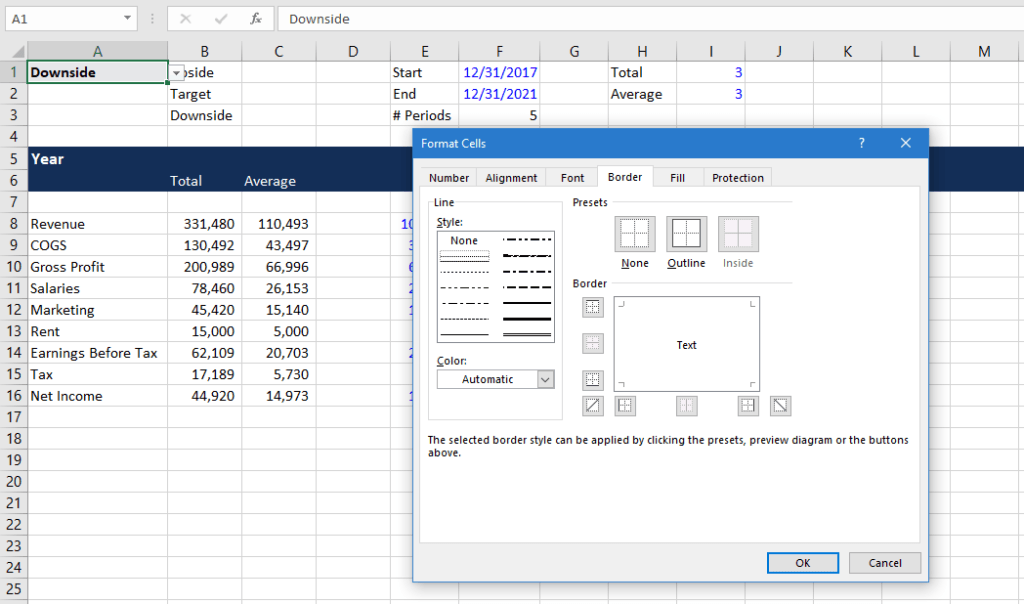
11. Press CTRL + 1 to format the drop-down list so we can easily locate it. Format the font to bold and change cell color.
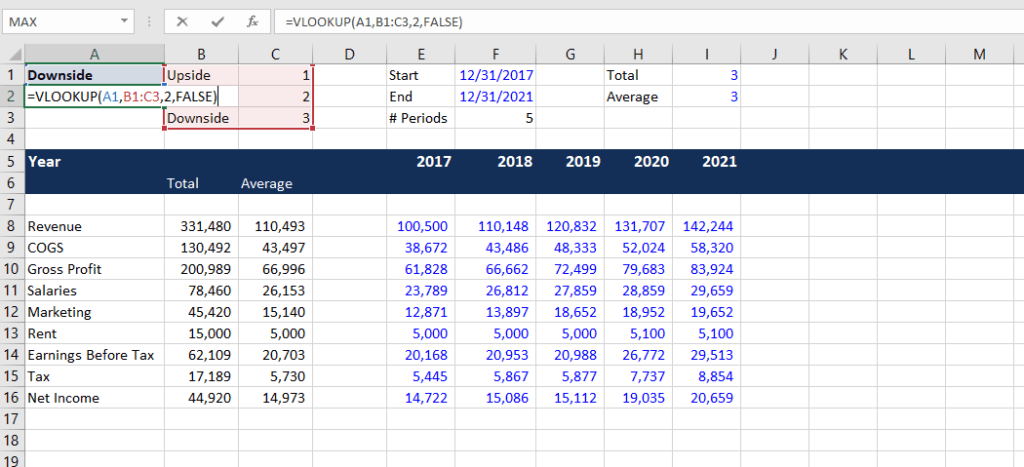
12. Number the three scenario cases in cells C1 to C3. In cell A2, use the VLOOKUP function to match the scenario name in the drop-down list to the case number. Enter the formula =VLOOKUP(A1,B1:C3,2,FALSE).
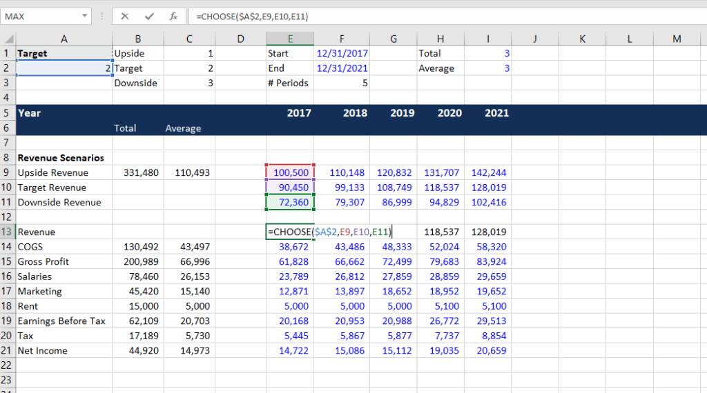
13. Now, we’ll insert some rows below revenue to show the three scenarios. At cell A9, press ALT + I + R four times to insert four new rows. Name them Upside Revenue, Target Revenue, and Downside Revenue. We will input some numbers for each of the scenarios in cells E8 to I10.
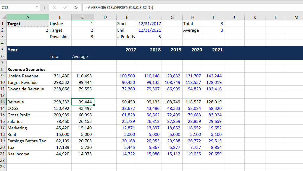
14. Row 13 is our live revenue numbers. In cell E13, use the CHOOSE function =CHOOSE($A$2,E9,E10,E11). The function allows us to create a dynamic revenue line which chooses the right option according to the scenario selected. Change the font to black, press SHIFT + right arrow then CTRL + R to copy formulas to the right.
15. Fill out the cells B10 to C11 by pressing CTRL + D. Copy and paste formulas from cell B11 and C11 to B13 and C13.
16. Now, we want to link the total and average label to the number of periods indicated in cells I1 and I2. In cell B6, enter =I1&”-Yr Total” so the total label displays “3-Yr Total” where the number is dynamic. For the average label, enter =I2&”-Yr Avg”.
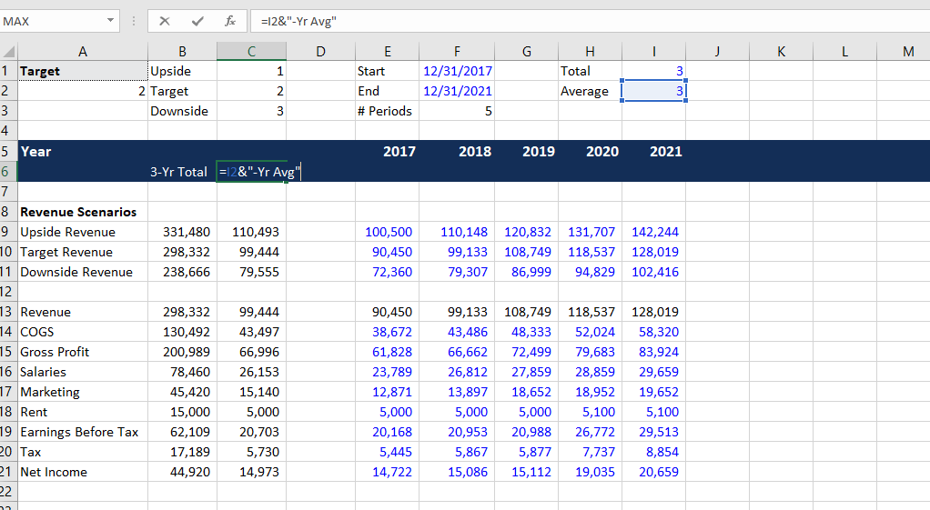
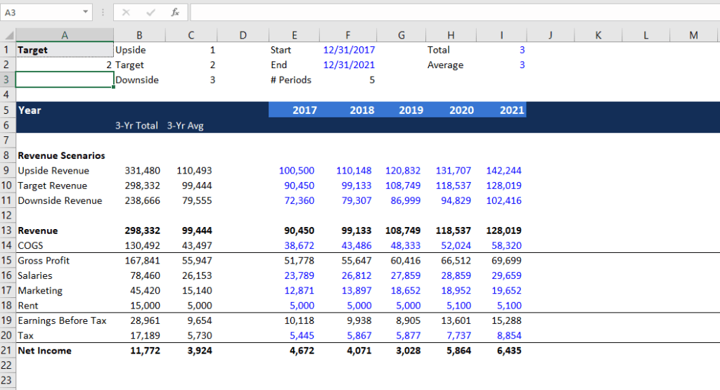
17. Finally, do a bit of formatting to the model. Change gross profits, earnings before taxes, and net income to formulas so they are all linked up. Your final model might look something like this:
CFI is the official provider of the global Financial Modeling & Valuation Analyst (FMVA)™ certification program, designed to help anyone become a world-class financial analyst. To keep advancing your career, the additional CFI resources below will be useful:
Below is a break down of subject weightings in the FMVA® financial analyst program. As you can see there is a heavy focus on financial modeling, finance, Excel, business valuation, budgeting/forecasting, PowerPoint presentations, accounting and business strategy.
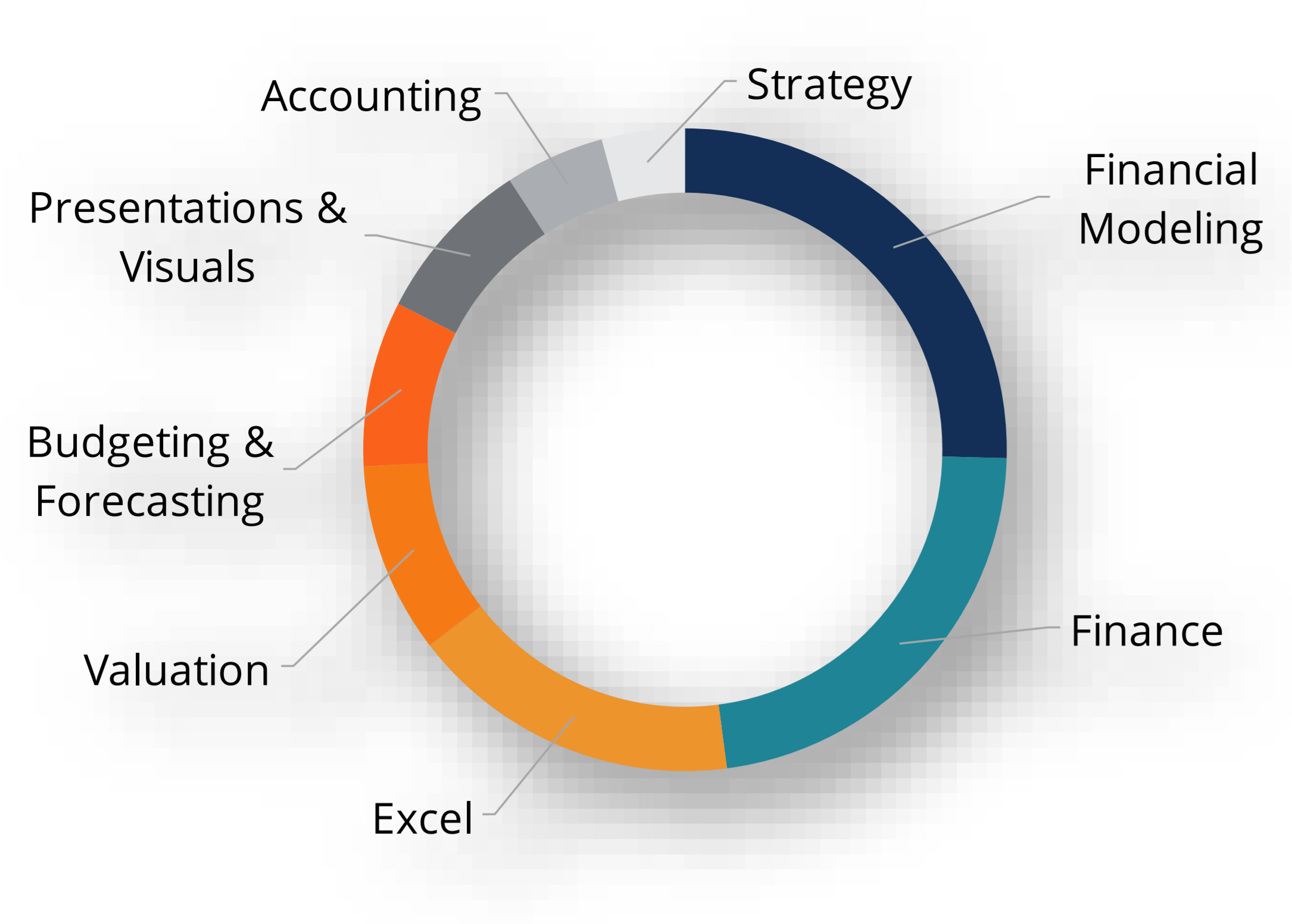
A well rounded financial analyst possesses all of the above skills!
CFI is the global institution behind the financial modeling and valuation analyst FMVA® Designation. CFI is on a mission to enable anyone to be a great financial analyst and have a great career path. In order to help you advance your career, CFI has compiled many resources to assist you along the path.
In order to become a great financial analyst, here are some more questions and answers for you to discover:
To master the art of Excel, check out CFI’s Excel Crash Course, which teaches you how to become an Excel power user. Learn the most important formulas, functions, and shortcuts to become confident in your financial analysis.

Launch CFI’s Excel Crash Course now to take your career to the next level and move up the ladder!


