VLOOKUP

What is VLOOKUP in Excel?

The VLOOKUP Function[1] in Excel is a tool for looking up a piece of information in a table or data set and extracting some corresponding data/information. In simple terms, the VLOOKUP function says the following to Excel: “Look for this piece of information (e.g., bananas), in this data set (a table), and tell me some corresponding information about it (e.g., the price of bananas)”.

Learn how to do this step by step in our Free Excel Crash Course!

VLOOKUP Formula

=VLOOKUP(lookup_value, table_array, col_index_num, [range_lookup])

To translate this to simple English, the formula is saying, “Look for this piece of information, in the following area, and give me some corresponding data from another column”.

The VLOOKUP function uses the following arguments:

1. Lookup_value (required argument) – Lookup_value specifies the value that we want to look up in the first column of a table. For example, if the data is in columns A through C, then the Lookup_value must be in column A.
2. Table_array (required argument) – The table array is the data array that is to be searched. The VLOOKUP function searches for the Lookup_value in the left-most column of this array. You can use a named range or a table, and you can use names in the argument instead of cell references.
3. Col_index_num (required argument) – This is an integer, specifying the column number of the supplied table_array, that you want to return a value from. The first column in the table_array is column 1, the second column is column 2, etc. 
4. Range_lookup (optional argument) – This defines what this function should return in the event that it does not find an exact match to the lookup_value. The argument can be set to TRUE or FALSE, which means:
   • TRUE – Approximate match, that is, if an exact match is not found, use the closest match to the lookup_value. By selecting TRUE, VLOOKUP assumes the first column in the table is sorted either numerically or alphabetically, and will then search for the closest value.
   • FALSE – Exact match, that is, if an exact match not found, then it will return an error.
   • You may also type 1 for TRUE or 0 for FALSE. If neither TRUE or FALSE is selected, Excel defaults to TRUE.

How to use VLOOKUP in Excel

Step 1: Organize the data

The first step to effectively using the VLOOKUP function is to make sure your data is well organized and suitable for using the function.

VLOOKUP works in a left-to-right order, so you need to ensure that the information you want to look up is to the left of the corresponding data you want to extract.

For example:

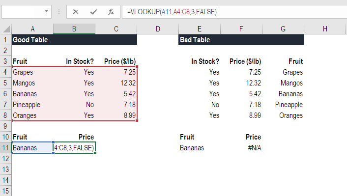
In the above VLOOKUP example, you will see that the “good table” can easily run the function to look up “Bananas” and return the price since Bananas are located in the left-most column.  In the “bad table” example you’ll see there is an error message, as the columns are not in the right order.

This is one of the major drawbacks of VLOOKUP, and for this reason, it’s highly recommended to use INDEX MATCH instead of VLOOKUP.

Step 2: Tell the function what to lookup

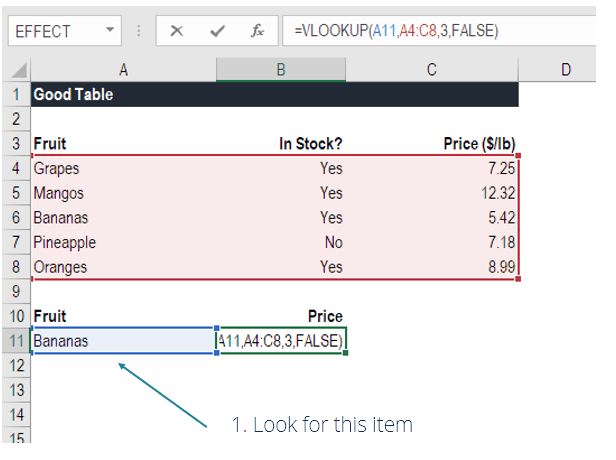
In this step, we tell Excel what to look for. We start by typing the formula “=VLOOKUP(“ and then select the cell that contains the information we want to lookup. In this case, it’s the cell that contains “Bananas”.

Step 3: Tell the function where to look

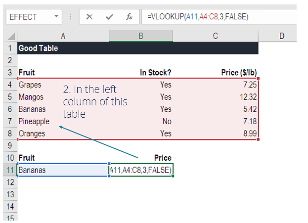
In this step, we select the table where the data is located, and tell Excel to search in the left-most column for the information we selected in the previous step.

For example, in this case, we highlight the whole table from column A to column C. Excel will look for the information we told it to look up in column A.

Step 4: Tell Excel what column to output the data from

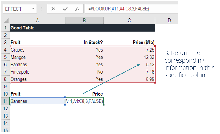
In this step, we need to tell Excel which column contains the data that we want to have as an output from the VLOOKUP. To do this, Excel needs a number that corresponds to the column number in the table.

In our example, the output data is located in the 3^rd column of the table, so we enter the number “3” in the formula.

Step 5: Exact or approximate match

This final step is to tell Excel if you’re looking for an exact or approximate match by entering “True” or “False” in the formula.

In our VLOOKUP example, we want an exact match (“Bananas”), so we type “FALSE” in the formula. If we instead used “TRUE” as a parameter, we would get an approximate match. Alternatively, if we didn’t make any selection then Excel assumes “TRUE” has been entered.

An approximate match would be useful when looking up an exact figure that might not be contained in the table, for example, if the number 2.9585. In this case, Excel will look for the number closest to 2.9585, even if that specific number is not contained in the dataset.  This will help prevent errors in the VLOOKUP formula.

Learn how to do this step by step in our Free Excel Crash Course!

VLOOKUP in financial modeling and financial analysis

VLOOKUP formulas are often used in financial modeling and other types of financial analysis to make models more dynamic and incorporate multiple scenarios.

For example, imagine a financial model that included a debt schedule, where the company had three different scenarios for the interest rate: 3.0%, 4.0%, and 5.0%. The VLOOKUP function could look for a chosen scenario: low, medium or high, and output the corresponding interest rate into the financial model.

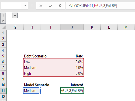
As you can see in the example above, an analyst can select the Medium scenario and the VLOOKUP will return 4.0%.

Things to remember about the VLOOKUP Function

Here is an important list of things to remember about the Excel VLOOKUP Function:

1. When range_lookup is omitted, the VLOOKUP function will allow a non-exact match, but it will use an exact match if one exists.
2. The biggest limitation of the function is that it always looks right. It will get data from the columns to the right of the first column in the table.
3. If the lookup column contains duplicate values, VLOOKUP will match the first value only.
4. The function is not case-sensitive.
5. Suppose there’s an existing VLOOKUP formula in a worksheet. In that scenario, formulas may break if we insert a column in the table. This is so because a hard-coded column index value doesn’t change automatically when columns are inserted or deleted. An analyst can get around this by making sure the column index value changes dynamically. If set up properly the MATCH function can do this (the COLUMNS function may also be helpful to create dynamic column index values).
6. VLOOKUP allows the use of wildcards, e.g., an asterisk (*) or a question mark (?). The ? matches any single character, while the * matches any sequence of characters.
7. Suppose in the table we are working with the function contains numbers entered as text. If we are simply retrieving numbers as text from a column in a table, then VLOOKUP will work fine. However, if the first column of the table contains numbers entered as text, we will get an #N/A! error if the lookup value is not also in text form.
8. #N/A! error – Occurs if the VLOOKUP function fails to find a match to the supplied lookup_value.
9. #REF! error – Occurs if either:
   • The col_index_num argument is greater than the number of columns in the supplied table_array; or
   • The formula attempted to reference cells that do not exist.
10. #VALUE! error – Occurs if either:
    • The col_index_num argument is less than 1 or is not recognized as a numeric value; or
    • The range_lookup argument is not recognized as one of the logical values TRUE or FALSE.
11. #NAME! error – Occurs if there is text used as the lookup_value and the text is not in quotes. For example, #NAME! would be returned if the formula VLOOKUP(Bananas,A4:C8,3,FALSE) was entered. To correct this, enter the formula like this: VLOOKUP(“Bananas”,A4:C8,3,FALSE). However, it’s still a better practice for the lookup_value to be a cell reference containing the proper criteria.

Additional Resources

This has been a guide to the VLOOKUP function, how to use it, and how it can be incorporated into financial modeling in Excel.

Even though it’s a great function, as mentioned above, we highly recommend using INDEX MATCH instead, as this combination of functions can search in any direction, not just left to right. To learn more, see our guide to INDEX MATCH. Additionally, a few years ago Excel introduced the XLOOKUP function, which is an improvement on VLOOKUP and matches up well with the versatility of INDEX MATCH.

To keep learning and developing your skills, check out these additional CFI resources:

• Free Excel Fundamentals Course
• Advanced Excel Formulas List
• Excel Keyboard Shortcuts
• IF with AND Functions
• Financial Modeling Guide
• See all Excel resources