Get Certified for
Business Intelligence (BIDA®)
Develop analytical superpowers by learning how to use programming and data analytics tools such as VBA, Python, Tableau, Power BI, Power Query, and more.
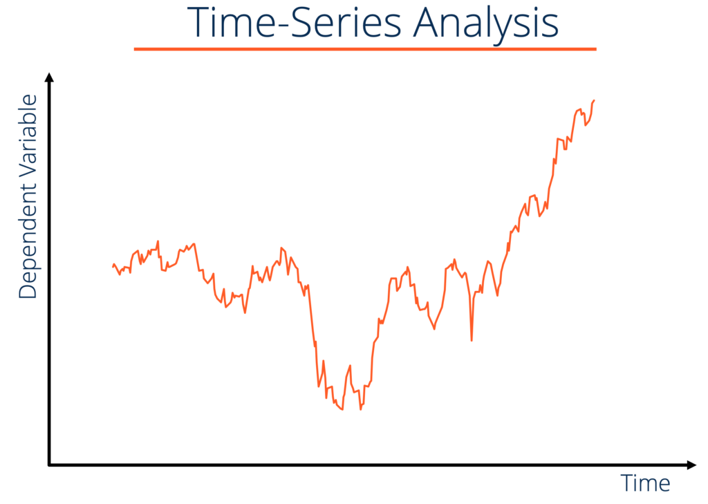
The analysis of a variables change over a period of time
Time series data analysis is the analysis of datasets that change over a period of time. Time series datasets record observations of the same variable over various points of time. Financial analysts use time series data such as stock price movements, or a company’s sales over time, to analyze a company’s performance.
Examples of time series datasets include:
Unlike cross-sectional data analysis, time series data analysis cannot make use of the random sampling framework. This makes time series data analysis much more complex and computationally demanding than cross-sectional data analysis. Random sampling cannot be used because the past values of a variable are almost always highly correlated with the present value of that variable.
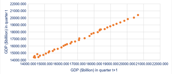
For example, the GDP of the US in the fourth quarter of 2017 is highly correlated with the GDP in the third quarter of 2017. The degree of correlation is much higher than the correlation across economic entities at the same point in time.
The correlation coefficient between the US GDP in the current quarter and the US GDP in the previous quarter for the period 2008 to 2018 is 0.998. The correlation coefficient between the US GDP in the current year and the US GDP in the previous year for the period 2008 to 2018 is 0.992.
The majority of economic analysis involves the study of intertemporal causal claims. Examples include:
Consider the test scores example: Suppose there is some policy instrument (e.g., increasing the teacher-student ratio) that can be used to increase Grade 7 test scores by 1%. Such a policy change is likely to be very expensive, and a policymaker who only looks at Grade 7 test scores might not implement the policy.
However, suppose a 1% increase in Grade 7 test scores is associated with a 0.5% increase in Grade 8 test scores. This additional benefit may make implementing the policy worthwhile.
Thank you for reading CFI’s guide to Time Series Data Analysis. To keep advancing your career, the additional CFI resources below will be useful:


