Get Certified for
Business Intelligence (BIDA®)
Develop analytical superpowers by learning how to use programming and data analytics tools such as VBA, Python, Tableau, Power BI, Power Query, and more.
The degree of correlation of the same variables between two successive time intervals
Autocorrelation refers to the degree of correlation of the same variables between two successive time intervals. It measures how the lagged version of the value of a variable is related to the original version of it in a time series.
Autocorrelation, as a statistical concept, is also known as serial correlation. It is often used with the autoregressive-moving-average model (ARMA) and autoregressive-integrated-moving-average model (ARIMA). The analysis of autocorrelation helps to find repeating periodic patterns, which can be used as a tool for technical analysis in the capital markets.
In many cases, the value of a variable at a point in time is related to the value of it at a previous point in time. Autocorrelation analysis measures the relationship of the observations between the different points in time, and thus seeks a pattern or trend over the time series. For example, the temperatures on different days in a month are autocorrelated.
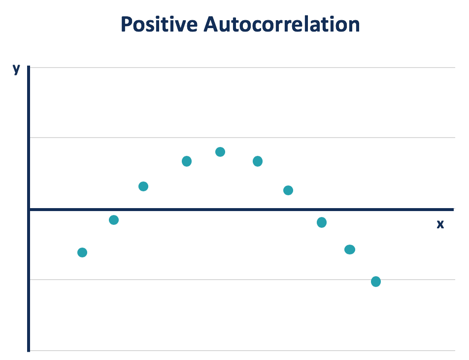
Similar to correlation, autocorrelation can be either positive or negative. It ranges from -1 (perfectly negative autocorrelation) to 1 (perfectly positive autocorrelation). Positive autocorrelation means that the increase observed in a time interval leads to a proportionate increase in the lagged time interval.
The example of temperature discussed above demonstrates a positive autocorrelation. The temperature the next day tends to rise when it’s been increasing and tends to drop when it’s been decreasing during the previous days.
The observations with positive autocorrelation can be plotted into a smooth curve. By adding a regression line, it can be observed that a positive error is followed by another positive one, and a negative error is followed by another negative one.
Conversely, negative autocorrelation represents that the increase observed in a time interval leads to a proportionate decrease in the lagged time interval. By plotting the observations with a regression line, it shows that a positive error will be followed by a negative one and vice versa.

Autocorrelation can be applied to different numbers of time gaps, which is known as lag. A lag 1 autocorrelation measures the correlation between the observations that are a one-time gap apart. For example, to learn the correlation between the temperatures of one day and the corresponding day in the next month, a lag 30 autocorrelation should be used (assuming 30 days in that month).
The Durbin-Watson statistic is commonly used to test for autocorrelation. It can be applied to a data set by statistical software. The outcome of the Durbin-Watson test ranges from 0 to 4. An outcome closely around 2 means a very low level of autocorrelation. An outcome closer to 0 suggests a stronger positive autocorrelation, and an outcome closer to 4 suggests a stronger negative autocorrelation.
It is necessary to test for autocorrelation when analyzing a set of historical data. For example, in the equity market, the stock prices on one day can be highly correlated to the prices on another day. However, it provides little information for statistical data analysis and does not tell the actual performance of the stock.
Therefore, it is necessary to test for the autocorrelation of the historical prices to identify to what extent the price change is merely a pattern or caused by other factors. In finance, an ordinary way to eliminate the impact of autocorrelation is to use percentage changes in asset prices instead of historical prices themselves.
Although autocorrelation should be avoided in order to apply further data analysis more accurately, it can still be useful in technical analysis, as it looks for a pattern from historical data. The autocorrelation analysis can be applied together with the momentum factor analysis.
A technical analyst can learn how the stock price of a particular day is affected by those of previous days through autocorrelation. Thus, he can estimate how the price will move in the future.
If the price of a stock with strong positive autocorrelation has been increasing for several days, the analyst can reasonably estimate the future price will continue to move upward in the recent future days. The analyst may buy and hold the stock for a short period of time to profit from the upward price movement.
The autocorrelation analysis only provides information about short-term trends and tells little about the fundamentals of a company. Therefore, it can only be applied to support the trades with short holding periods.
Thank you for reading CFI’s guide to Autocorrelation. To keep learning and advancing your career, the following resources will be helpful:


