Central Limit Theorem

What is the Central Limit Theorem (CLT)?

The Central Limit Theorem (CLT) is a statistical concept that states that the sample mean distribution of a random variable will assume a near-normal or normal distribution if the sample size is large enough. In simple terms, the theorem states that the sampling distribution of the mean approaches a normal distribution as the size of the sample increases, regardless of the shape of the original population distribution.

As the user increases the number of samples to 30, 40, 50, etc., the graph of the sample means will move towards a normal distribution. The sample size must be 30 or higher for the central limit theorem to hold.

One of the most important components of the theorem is that the mean of the sample will be the mean of the entire population. If you calculate the mean of multiple samples of the population, add them up, and find their average, the result will be the estimate of the population mean.

The same applies when using standard deviation. If you calculate the standard deviation of all the samples in the population, add them up, and find the average, the result will be the standard deviation of the entire population.

How Does the Central Limit Theorem Work? 

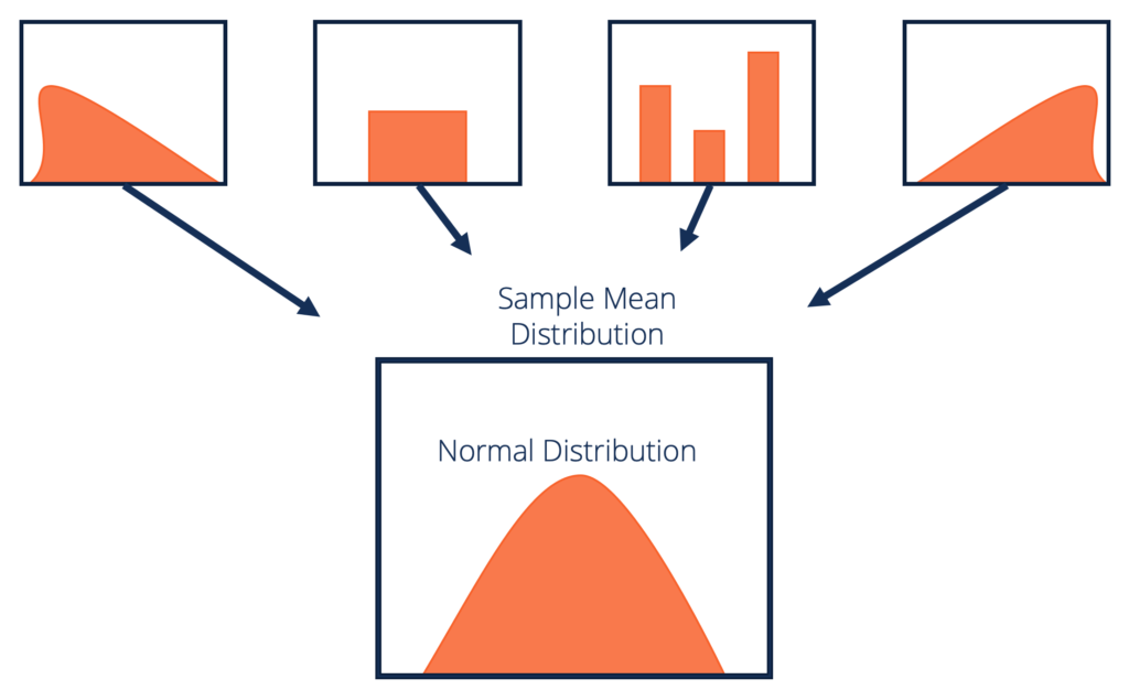
The central limit theorem forms the basis of the probability distribution. It makes it easy to understand how population estimates behave when subjected to repeated sampling. When plotted on a graph, the theorem shows the shape of the distribution formed by means of repeated population samples.

As the sample sizes get bigger, the distribution of the means from the repeated samples tends to normalize and resemble a normal distribution. The result remains the same regardless of what the original shape of the distribution was. It can be illustrated in the figure below:

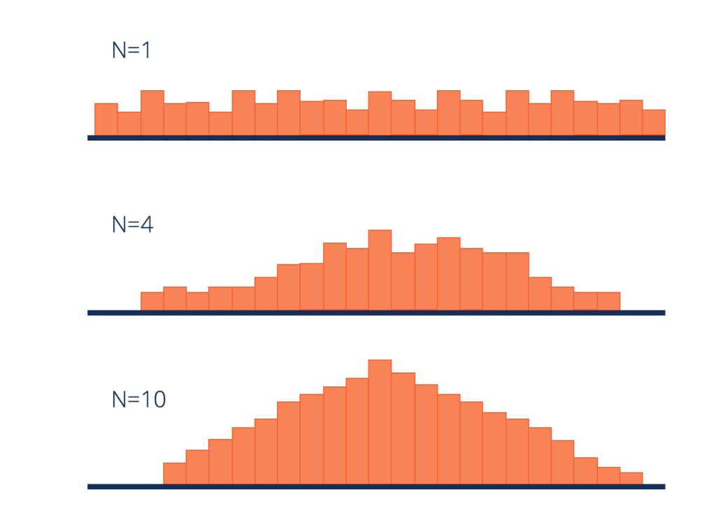
From the figure above, we can deduce that despite the fact that the original shape of the distribution was uniform, it tends towards a normal distribution as the value of n (sample size) increases.

Apart from showing the shape that the sample means will take, the central limit theorem also gives an overview of the mean and variance of the distribution. The sample mean of the distribution is the actual population mean from which the samples were taken.

The variance of the sample distribution, on the other hand, is the variance of the population divided by n. Therefore, the larger the sample size of the distribution, the smaller the variance of the sample mean.

Example of Central Limit Theorem

An investor is interested in estimating the return of ABC stock market index that is comprised of 100,000 stocks. Due to the large size of the index, the investor is unable to analyze each stock independently and instead chooses to use random sampling to get an estimate of the overall return of the index.

The investor picks random samples of the stocks, with each sample comprising at least 30 stocks. The samples must be random, and any previously selected samples must be replaced in subsequent samples to avoid bias.

If the first sample produces an average return of 7.5%, the next sample may produce an average return of 7.8%. With the nature of randomized sampling, each sample will produce a different result. As you increase the size of the sample size with each sample you pick, the sample means will start forming their own distributions.

The distribution of the sample means will move toward normal as the value of n increases. The average return of the stocks in the sample index estimates the return of the whole index of 100,000 stocks, and the average return is normally distributed.

History of the Central Limit Theorem

The initial version of the central limit theorem was coined by Abraham De Moivre, a French-born mathematician. In an article published in 1733, De Moivre used the normal distribution to find the number of heads resulting from multiple tosses of a coin. The concept was unpopular at the time, and it was forgotten quickly.

However, in 1812, the concept was reintroduced by Pierre-Simon Laplace, another famous French mathematician. Laplace re-introduced the normal distribution concept in his work titled “Théorie Analytique des Probabilités,” where he attempted to approximate binomial distribution with the normal distribution.

The mathematician found that the average of independent random variables, when increased in number, tends to follow a normal distribution.  At that time, Laplace’s findings on the central limit theorem attracted attention from other theorists and academicians.

Later in 1901, the central limit theorem was expanded by Aleksandr Lyapunov, a Russian mathematician. Lyapunov went a step ahead to define the concept in general terms and prove how the concept worked mathematically. The characteristic functions that he used to provide the theorem were adopted in modern probability theory.

Related Readings

Thank you for reading CFI’s guide to Central Limit Theorem. To keep learning and advancing your career, the additional CFI resources below will be useful:

• Bayes’ Theorem
• Central Tendency
• Law of Large Numbers
• Total Probability Rule
• See all data science resources