Get Certified for
Business Intelligence (BIDA®)
Develop analytical superpowers by learning how to use programming and data analytics tools such as VBA, Python, Tableau, Power BI, Power Query, and more.
One of R's strengths remains the ability to run a variety of statistical tests
Some of the strongest use cases for R, a popular programming language that is widely used for data science and data analysis, have to do with the packages and tools that have been built around the language and that take advantage of its extensibility and open-source availability. Its base capability is known as Base R, but R possesses many different packages that extend this functionality. This includes a wide variety of statistical functionality, such as linear modeling, classification, clustering, statistical tests, time-series analysis, and graphing.
Some of the primary benefits of using R for data science include:
R was originally developed as a programming language for statistical analysis and one of its strengths remains the ability to run a variety of statistical tests. The core R functionality that is available once R is downloaded is known as Base R. This included programming basics like operators and variable definition, as well as a suite of mathematical and statistical functions.
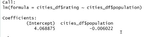
A common statistical test is fitting a linear regression model. This can be done with the Base R function of lm(). The syntax for fitting a linear model looks like this:
lm(rating ~ population, data = cities_df)
![]()
The first argument of the function is the formula used to fit the model. The tilde character (~) separates the dependent variable on the left, what we are trying to predict or explain, from the independent variable on the right, what we are using to explain the dependent variable. In this case, we are trying to use the population column to explain the rating column.
Both of these columns are from the data set defined in the second “data” argument. In this example, the rating and population column are contained in the cities dataframe.
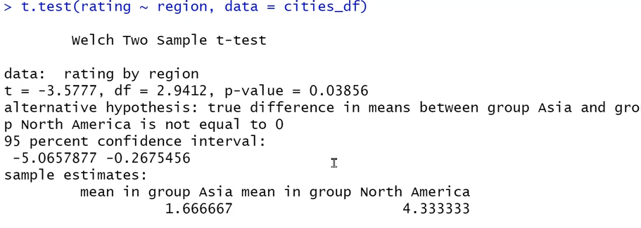
Another common statistical test is the t-test, which we can use to compare the means of two columns. A t-test can allow us to determine if the difference between the means of two groups are statistically significant. In the following example, we are trying to determine if the mean in rating between two different regions of the data set are significantly different.
t.test(rating ~ region, data = cities_df)
![]()
The final example of a statistical test made easy in Base R is an analysis of variance. This function is similar to the t-test, but, instead of comparing the mean of two samples, it lets us compare the means of multiple samples. In the following example, we are trying to determine if the mean in rating between three different countries of the data set are significantly different.
output_aov <- aov(rating ~ country, data = cities_df)

summary(output_aov)
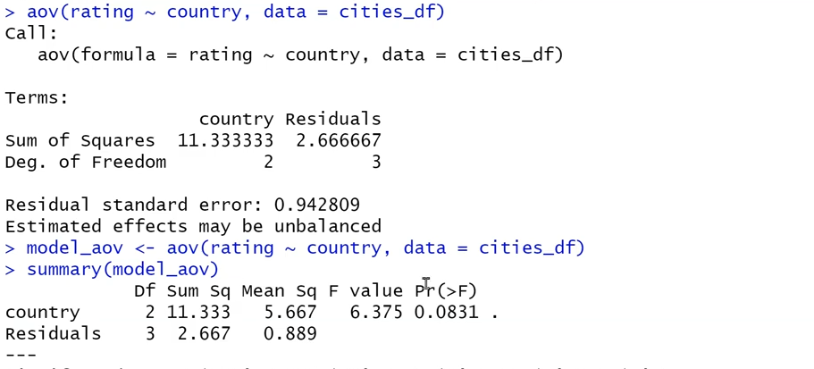
In the second part of the above example, we save the output of the aov() function into a variable, model_aov, then use the summary function on the model. We see the sum of the squares, the degrees of freedom, and the residual standard error. Ultimately this makes the output easier to read and gives us more insight into the results of the statistical tests.
The tidyverse is a collection of R packages designed for data science. All packages in the tidyverse share a consistent design philosophy, grammar, and data structures.
The tidyverse provides intuitive and readable functions that can be combined together across packages. This includes the ability to write code left to right with functions and function arguments that are readily consumable: named to explain what they do.
The tidyverse can be broadly split into two different parts. The core tidyverse includes the packages that we’re most likely to use in all of our data analysis projects. Outside of the core packages, the tidyverse also includes other packages with more specific use cases.
There are tidyverse packages for:
The readr package can be used to import rectangular data from delimited files. One of the most common data sources are .csv files, so the readr package provides a fast and intuitive way to import the data from these files. Similarly, the readxl package can be used to import data from Excel. The functions follow a similar philosophy to those in readr, with added arguments to connect to certain sheets and define which cells to import.
The tidyr package can be used to clean and organize data so that it is tidy. This means that every column in a dataset equates to a single variable, every row equates to a single observation, and every cell contains only one value. The package includes functions to pivot and unpivot data as well as deal with missing values.
The dplyr package provides a set of functions to manipulate data. These functions cover the most common data transformations needed to analyze data:
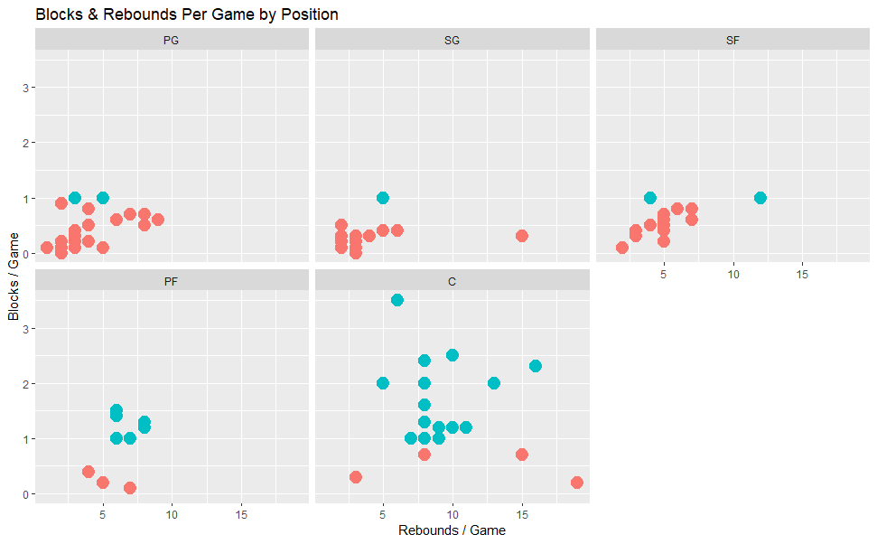
The ggplot2 package is used to create data visualizations based on the philosophy of the grammar of graphics. The grammar of graphics is useful because it provides a framework to think about our plots, which will help us focus on developing the plots themselves — rather than just the R code syntax. The three foundational pieces to create and define a plot are:

For data, we select the specific data set to visualize. Aesthetics map columns from our data to specific attributes of a plot. A common aesthetic that is defined in almost all plots are the x- and y-axis. We need to define which columns from the data set are mapped to the plot axis. Geoms define what type of plot to generate — such as a line chart or a scatter chart. A plot with the same data and aesthetics can look different depending on the geom selected.
Pipes %>% allow multiple functions to be combined together in the tidyverse. The output from the previous functions is ‘piped’ into the data argument of the next function. This allows users to write more concise code by combining multiple functions in one code chunk.
The tidymodels meta package is a collection of packages to create models that follow tidy principles. The package shares common APIs and philosophies that the tidyverse packages use for data analysis.
Similar to the tidyverse, tidymodels consists of both core and specialized packages. Three core packages from tidymodels are:
The rsample package provides functions to create different types of samples and resamples, as well as the corresponding classes for their analysis. Creating resamples is important in modeling to estimate the sampling distribution of a statistic and to estimate the model performance using a holdout set.
The recipes package provides a set of functions for feature engineering and data pre-processing ahead of modeling. It is similar to the dplyr package from the tidyverse, but the manipulation functions are more specific to data modeling, such as one hot encoding and scaling variables.
The yardstick package is used to measure model performance. It produces output that is tidy and can be interacted with using similar functionality to the tidyverse packages. We can pipe the output generated by the yardstick package into functions that help us better understand what the model does well and what can be improved.
The features and functionality of the RStudio IDE allows coding with R to be quicker, more efficient, and more convenient. This leads to a better user experience when conducting data analysis, and allows users to focus on what matters — analyzing data and applying expertise.
The RStudio IDE consists of four main panes:
The console is where R code is run and executed. The output generated by the code appears in the console. We can also write R code directly in the console as well, so the input code and resulting output can appear in the same place.

A better practice to help us write, maintain, and edit R code is to create an R Script. R Scripts define the code that is then run in the console. These scripts can be saved with a .r file extension.

Managing the R Scripts for a project is done in the Files pane. The Files tab lists all external files and directories in the current working directory on your computer. It works like the file explorer or finder. The Plots tab is where all the plots you create in R are displayed. The Packages tab lists all of the packages that you have installed on your computer. You can also install new packages and update existing packages by clicking on the Install and Update buttons respectively.
The Help tab displays the R help documentation for any package or function.The Environment tab displays all the objects that have been created in the current environment. These objects include functions that have been defined in an R Script or data sets that have been imported to clean and analyze.
There’s also an Import Dataset button which will import data saved in a variety of file formats. The History tab contains a list of all the commands you have entered into the R Console. The Connections tab allows you to connect to various data sources such as external databases.
Cheat sheets provide a quick overview of the common functions and arguments of tidyverse packages. They are available online, as well as directly in the RStudio IDE.
Connect what you just learned to a clear career path with CFI’s role‑based courses and certification programs.


