MIRR Function

What is the MIRR Function?

The MIRR Function[1] is categorized under Excel Financial functions. The function will provide the rate of return for an initial investment value and a series of net income values. MIRR uses a schedule of payments, including an initial investment and a series of net income payments, to calculate the compounded return, assuming the Net Present Value (NPV) of the investment is zero.

The function is very helpful in financial analysis for an investment, as it helps to calculate the return an investment will earn based on a series of mixed cash flows.

We can also use MIRR in financial modeling, although the common practice is to use IRR, as transactions are studied in isolation. MIRR is different from IRR because it helps set a different reinvestment rate for cash flows received. Thus, the MIRR function considers the initial cost of the investment and also the interest received on the reinvestment of cash, whereas the IRR function does not.

Formula

=MIRR(values, finance_rate, reinvest_rate)

The MIRR function uses the following arguments:

1. Values (required argument) – This is an array or a reference to cells that contain numbers. The numbers are a series of payments and income that incur negative values. Payments are represented by negative values and income by positive values.
2. Finance_rate (required argument) – The interest rate that is paid on the money that was used in the cash flows.
3. Reinvest_rate (required argument) – It is the interest that we receive on the cash flows as we reinvest them.

Notes on the arguments:

1. The argument value should contain at least one positive and one negative value to calculate MIRR.
2. The payment and income values should be in the sequence we want and with the correct signs, which is positive values for cash received and negative values for cash paid.
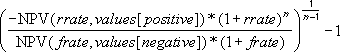
3. If n is the number of cash flows in values, frate is the finance_rate, and rrate is the reinvest_rate, the formula for MIRR is:

How to use the MIRR Function in Excel?

To understand the uses of the MIRR function, let’s consider a few examples:

Example 1

Let’s assume we need to choose one project from two given projects. The initial investment for both projects is the same. Year-wise, the cash flows are as follows:

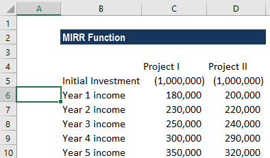
In the screenshot above, C5 and D5 are the initial investment amounts in Project I and Project II. Cells C6:C10 and D6:D10 show the cash inflows for Project I and Project II, respectively.

The finance rate and the reinvestment rate of the projects is 6% and 5%, respectively. The formulas to be used are as follows:

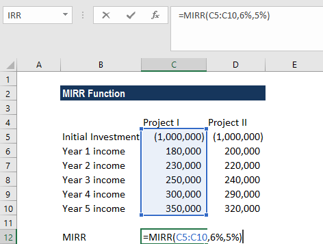
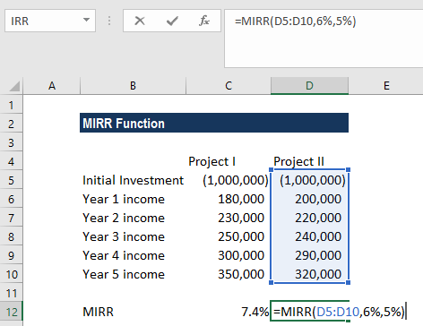
Remember that the initial investment needs to be in negative form, else the formula will return an error. The initial investment is a negative value, as it is an outgoing payment, and the income payments are represented by positive values.

We get the result below:

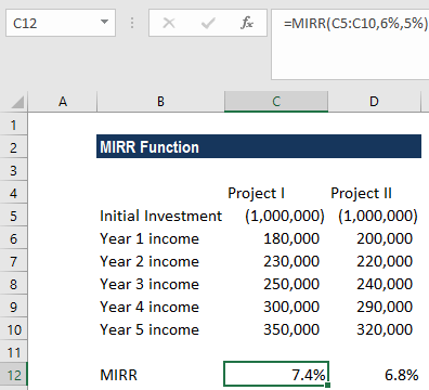
As we can see above, Project I is preferable because it shows a higher rate of return.

Things to remember about the MIRR Function

1. #DIV/0! error – Occurs when the given value array does not include at least one positive value and one negative value.
2. #VALUE! error – Occurs when any of the given arguments is non-numeric.

Click here to download the sample Excel file

Additional Resources

Thanks for reading CFI’s guide to the Excel MIRR function. By taking the time to learn and master Excel functions, you’ll significantly speed up your financial analysis. To learn more, check out these additional CFI resources:

• Excel Functions for Finance
• Advanced Excel Formulas Course
• Advanced Excel Formulas You Must Know
• Excel Shortcuts for PC and Mac
• See all Excel resources