Dynamic Financial Analysis
Use Excel formulas and functions in financial analysis
Dynamic Financial Analysis
This guide will teach you how to perform dynamic financial analysis in Excel using advanced formulas and functions.
INDEX, MATCH, and INDEX MATCH MATCH Functions
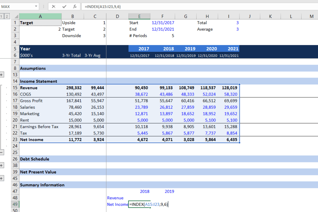
1. The INDEX function works similarly to the VLOOKUP function by returning a value in a table based on the intersection of a row and column position within that table. For example, say we want to find the net income for 2018 from the Income Statement section. In cell E49, we use the INDEX formula =INDEX(A15:I23,9,6) to look up the 9th row and 6th column in the income statement table to extract the net income value.
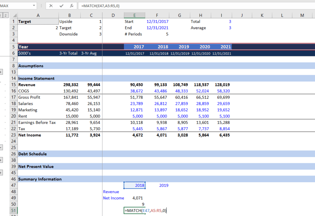
2. The MATCH function searches for a specified item in a range of cells and then returns the relative position of the item in the range. For example, suppose we want to find out the row and column where the 2018 net income is located in the Income Statement table. We can use the MATCH formula =MATCH(D49,A15:A23,0) to find the row position and =MATCH(E47,A5:R5,0) to find the column position.
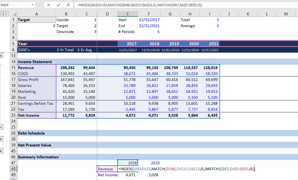
3. Combining the INDEX and MATCH functions, we can create a dynamic formula to search for the value we want from the Income Statement table. For example, assume we want to look up the revenue amount in 2018. In cell E48, enter =INDEX($A$15:I23,MATCH($D48,$A$15:$A$23,0),MATCH(E$47,$A$5:$R$5,0)). You can quickly look up a number in a specific year by changing the blue colored input.
Goal Seek (What-if Analysis)
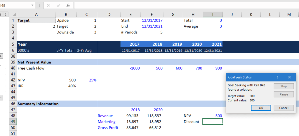
We can use the Goal Seek function to find out the results we are looking for. Suppose we want an NPV of 500 and we want to find out the discount rate. Let’s look at this form of dynamic financial analysis in action.
1. Press ALT + A + W + G to open the Goal Seek window. Set cell B42 (NPV) to 500 by changing C42 (discount rate). We then find out the discount rate has to be 25% in order to have an NPV of 500. Input 25% in cell I49.
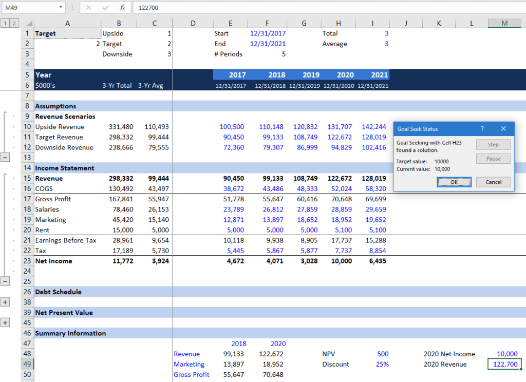
2. Another example of Goal Seek: Suppose we want to earn a net income of $10 million in 2020 and we want to figure out how much revenue we need to earn. Press ALT + A + W + G, set cell H23 (2020 net income) to 10,000 by changing cell H11 (target revenue). We need to earn $122.7 million in revenue to get $10 million net income. Input 122,700 in cell M49.
Dynamic Totals with INDIRECT and SUM Formulas
Recall from Parts I and II, we used the OFFSET function to create dynamic calculations by linking to some reference cells. We can perform a similar calculation using the INDIRECT formula along with other formulas such as SUM. For example, assume we want to sum up the free cash flows from cell E40 to I40. INDIRECT replaces the direct linking with the names of those cells.
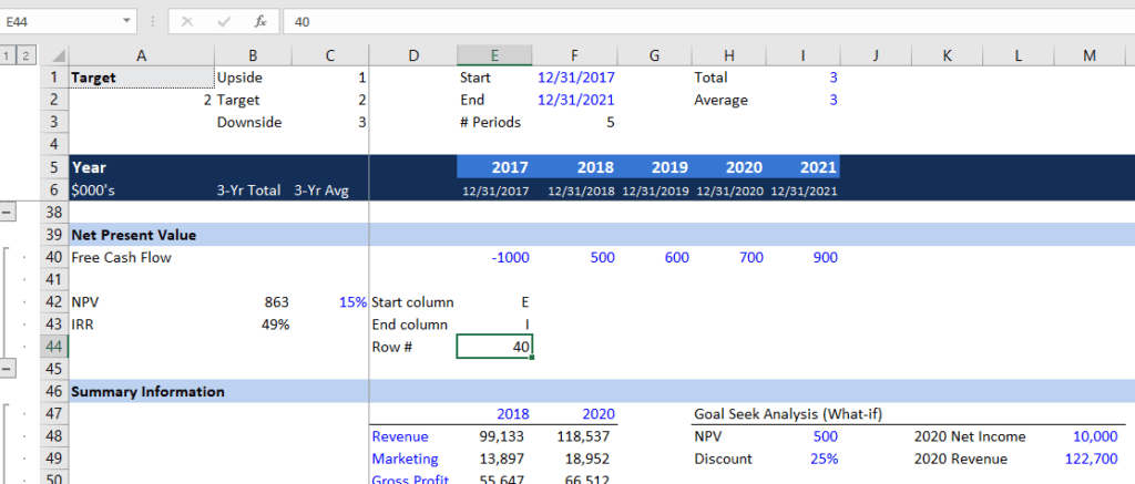
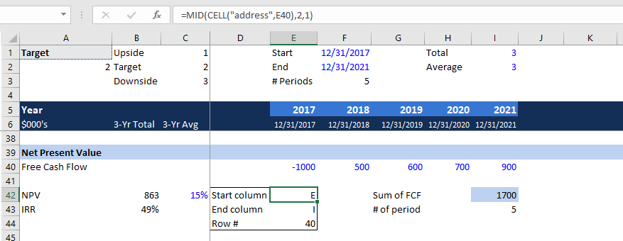
1. In cell D42 to D44, enter start column, end column, and row #. Then in cell E42 to E44, enter E as start column, I as end column, and 40 as row #.
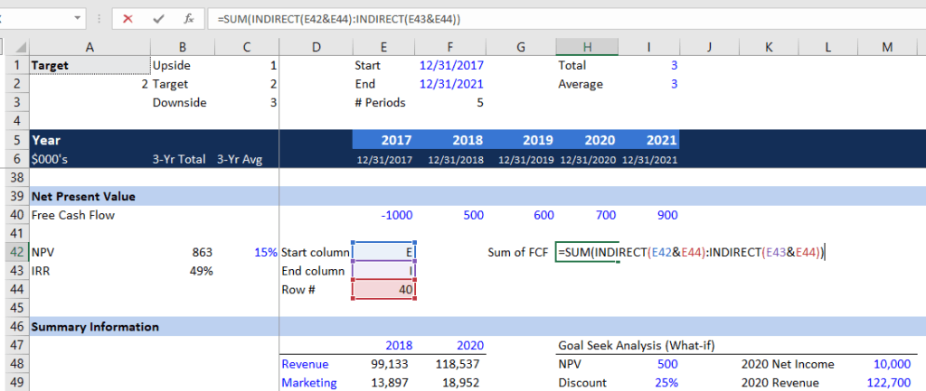
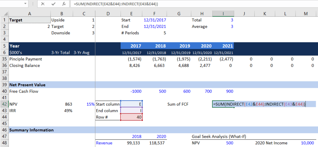
2. To calculate the sum of free cash flow (FCF), we can use the INDIRECT formula =SUM(INDIRECT(E42&E44):INDIRECT(E43&E44)). The formula takes the value from E42 to E44 to find the numbers being summed, making the SUM formula very dynamic.
CELL Function
Assume that you want to move the free cash flow values to another row. Instead of entering the row number every time the values are moved, you can use the CELL function to locate the values.
3. In cell E44, enter the CELL function =CELL(“row”,E40) so that the formula looks up for the FCF row number. You can use this formula to look for other things like file address or format.
COUNTA Function
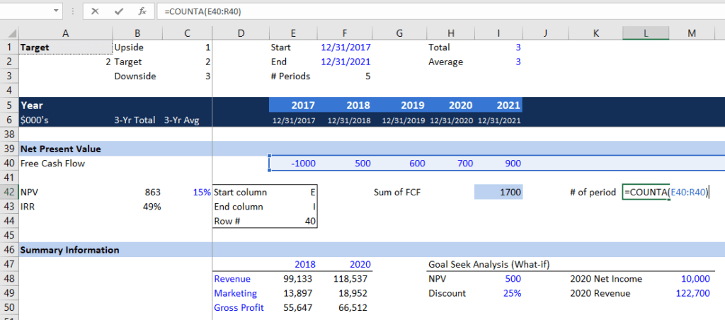
The COUNTA function returns all the cells that are not blank and is used to count cells that contain information.
4. In cell L42, enter the COUNTA function =COUNTA(E40:R40) to count the number of free cash flows. In a later section, we will see how the COUNTA function combined with other formulas can become a powerful tool in financial analysis.
MID Function
MID function returns a value from a cell. Say you want to extract the column information from cell E40. You can use the MID function to obtain the “E” value.
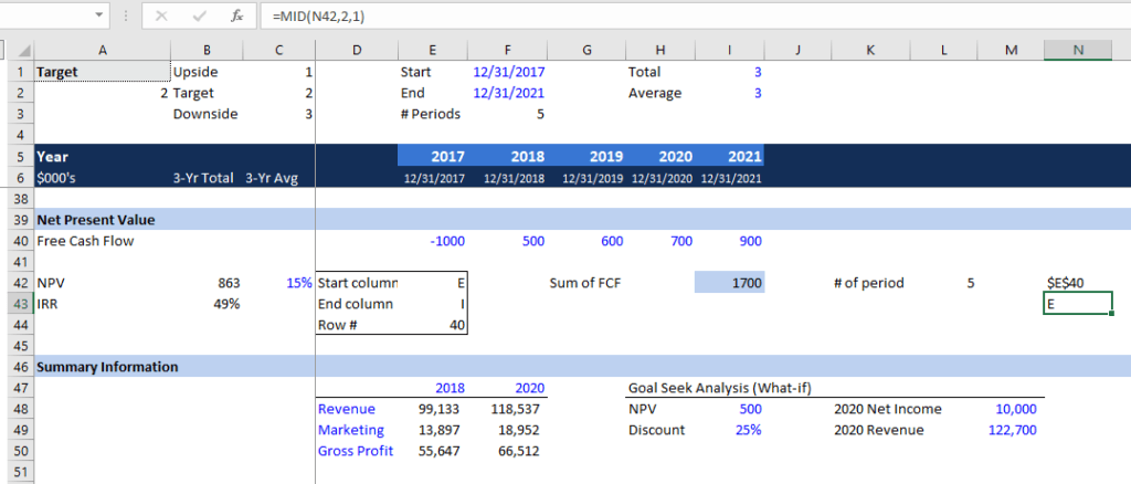
5. In cell N42, use the CELL function to find the address of the E40 =CELL(“address”,E40). The cell should display “$E$40”. Now in cell N43, enter the MID function to locate the column =MID(N42,2,1). This formula tells Excel to look at cell N42 and show one letter or number starting with the 2nd. You should see “E” in cell N43.
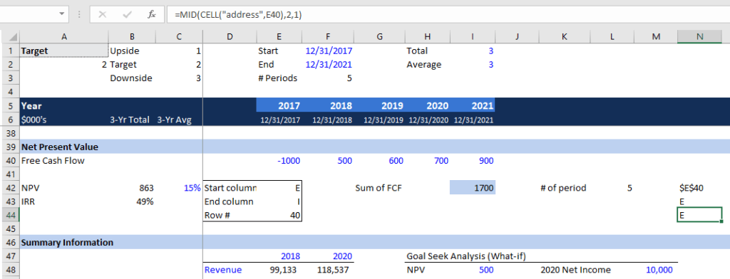
6. To combine the MID and CELL functions in one formula, you can simply type =MID(CELL(“address”,E40),2,1). It will give the same value “E”.
Combining CELL, COUNTA, MID and OFFSET in a Formula
Now we can combine the four functions to perform a very dynamic FCF calculation. Recall from the previous section, we combined the MID and CELL function to locate a cell value. We can now use that formula to find out the sum of FCF.
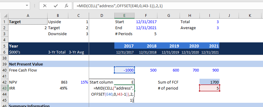
7. In cell E42, type the formula that we used in the last section: =MID(CELL(“address”,E40),2,1). Now the start column is correctly shown as “E”.
8. In cell E43, copy and paste the formula from E42. We need to make a little change to the formula so Excel picks up the end column “I”. Instead of putting E40 as the cell reference, we use the OFFSET function to locate the 5th FCF by linking to cell I43 (# of periods). The formula should look like =MID(CELL(“address”,OFFSET(E40,0,I43-1)),2,1).
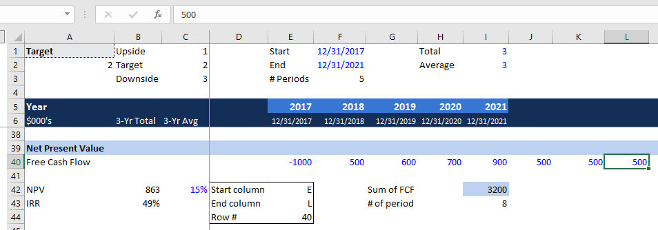
9. Excel will now automatically calculate the sum of FCF. You can freely adjust the number of FCFs in row 40.
Combining IF with AND and OR formulas
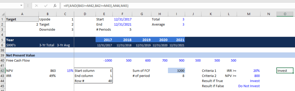
We can combine the IF, AND, and OR functions to make a decision based on some criteria. For example, assume we would like to make an investment if the IRR is greater than or equal to 20% and the NPV is greater than or equal to $800,000.
10. With all the criterion set up in place, we can use the IF and AND formulas to determine whether we should invest or not. In cell O42, enter =IF(AND(B43>=M42,B42>=M43),M44,M45). It tells us to invest because it meets both the IRR and NPV criteria.
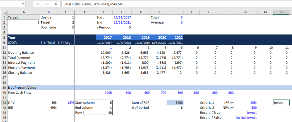
11. Let’s say we will invest if it meets either one of the two criteria. Instead of the AND function, we will use the OR formula. The formula in cell O42 should look like this: =IF(OR(B43>=M42,B42>=M43),M44,M45).
Summary of Key Formulas for Dynamic Financial Analysis
- INDEX formula for returning a value: =INDEX(table range, row #, column #)
- MATCH formula for returning relative position of an item: =MATCH(reference cell, table range, 0)
- INDEX MATCH MATCH formula to replace VLOOKUP: =INDEX(table range, MATCH(reference cell for row label, table range, 0), MATCH(reference cell for column label, table range, 0))
- INDIRECT formula to return a reference to a range: =INDIRECT(reference cells)
- CELL formula to locate the row number of a value: =CELL(“row”, cell #)
- COUNTA formula to count the number of cells with value: =COUNTA(cell range)
- MID formula to return a value from a cell: =MID(cell, start position, # values to include)
More Resources
Thank you for reading CFI’s guide to dynamic financial analysis. CFI is a global provider of financial analyst certification and career advancement for finance professionals. To learn more and expand your career, explore the additional relevant CFI resources below.
Analyst Certification FMVA® Program
Below is a break down of subject weightings in the FMVA® financial analyst program. As you can see there is a heavy focus on financial modeling, finance, Excel, business valuation, budgeting/forecasting, PowerPoint presentations, accounting and business strategy.
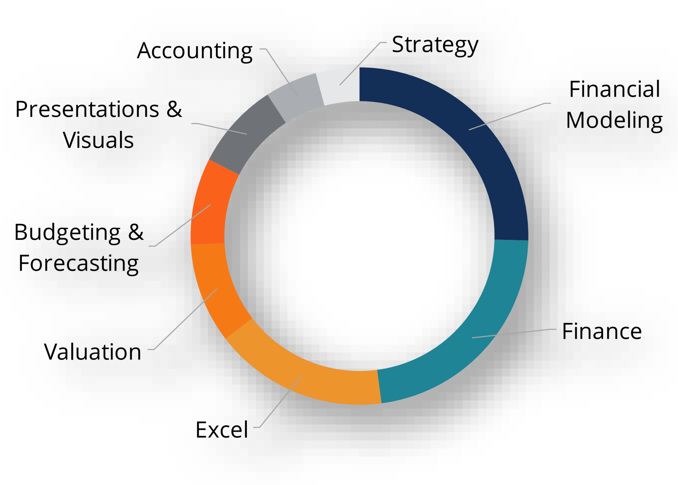
A well rounded financial analyst possesses all of the above skills!
Additional Questions & Answers
CFI is the global institution behind the financial modeling and valuation analyst FMVA® Designation. CFI is on a mission to enable anyone to be a great financial analyst and have a great career path. In order to help you advance your career, CFI has compiled many resources to assist you along the path.
In order to become a great financial analyst, here are some more questions and answers for you to discover:
- What is Financial Modeling?
- How Do You Build a DCF Model?
- What is Sensitivity Analysis?
- How Do You Value a Business?
Excel Tutorial
To master the art of Excel, check out CFI’s Excel Crash Course, which teaches you how to become an Excel power user. Learn the most important formulas, functions, and shortcuts to become confident in your financial analysis.

Launch CFI’s Excel Crash Course now to take your career to the next level and move up the ladder!


