Autonomous Expenditures
Expenditures that do not vary with the economy’s real level of income
What are Autonomous Expenditures?
Autonomous expenditures are expenditures that do not vary with the economy’s real level of income. They are considered necessary and are associated with the ability to maintain a state of autonomy at the individual or the government level.

Autonomous expenditures must be incurred regardless of the level of personal income and are mostly financed by personal savings and other credit mechanisms, such as loans and credit cards, when income levels are zero.
Government expenditure, exports, basic living expenses like food, shelter, etc. are examples of autonomous expenditures. These are mostly influenced by external factors such as trade policies, political uncertainties, interest rates, etc.
Summary
- Expenditures that do not vary with the economy’s real level of income are called autonomous expenditures.
- Autonomous expenditures are mostly influenced by external factors such as trade policies, political uncertainties, interest rates, etc.
- The SSM model emphasizes the role of autonomous demand growth in shaping the dynamics of the total output of an economy.
What are Induced Expenditures?
Induced expenditures are affected by changes in disposable income and demonstrate the wealth effect – the notion that consumers tend to spend more as their wealth grows. For instance, expenditure incurred on normal goods is considered to be induced.
Difference Between Autonomous and Induced Expenditures
Autonomous expenditure is represented by a horizontal line parallel to the x-axis, whereas the curve representing the induced aggregate expenditure is upward sloping and with a slope greater than zero.
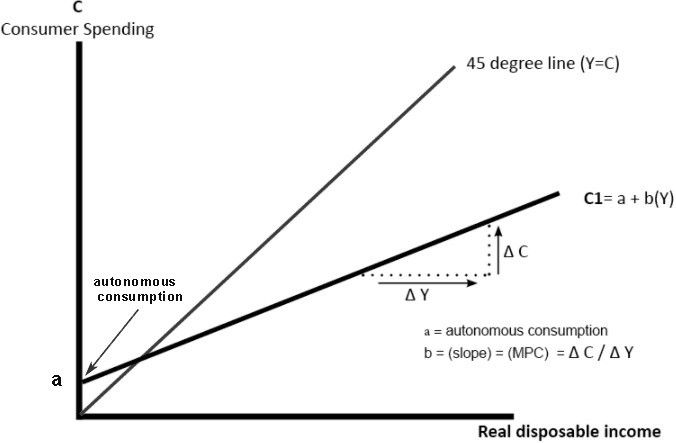
Consumption Function and Aggregate Expenditure
The Keynesian Consumption Function describes the functional relationship between total consumption and gross national income and symbolically, the relationship is represented as:
C = f(Y)
C = Cauto + MPC.Yd
Where:
- Cauto is autonomous consumption
- MPC is marginal propensity to consume
- Yd is disposable income
Aggregate Expenditure (AE) = Cauto + MPC.Yd + Iplanned + G + NX
= AEauto + MPC.Yd
The Sraffian Supermultiplier
The SSM model emphasizes the role of autonomous demand growth in shaping the dynamics of the total output of an economy. It rests on the following assumptions:
- The existence of non-capacity generating components of autonomous demand – exports, government expenditure, autonomous business expenditure, and autonomous consumption.
- Investment expenditure is not autonomous, even in the short term.
- Capitalist competition results in gradual changes in the marginal propensity to invest.
In the SSM model, the supply conditions of the economy determine capacity utilization in the long run. However, the growth rate of output and capital stock is determined by the growth rate of the non-capacity creating autonomous demand. The causality runs from autonomous demand to output through the supermultiplier.
As changes in autonomous demand are transmitted to output, changes in other variables like interest rate, propensity to invest, income distribution, etc., that play a more vital role in driving demand, exert only a temporary effect on economic growth. Over time, the effects fade away.
Since the system, by assumption, moves towards normal capacity utilization, autonomous expenditure drives long-run economic growth. Thus, the whole system grows at the rate of growth of autonomous expenditure.
How Autonomous is “Autonomous Demand” in the Long Run?
For instance, during the Greek Financial Crisis, extreme austerity measures imposed by the Greek government were predicted to have a long-run impact on the economy’s ability to grow. And this is exactly what happened.
Even in a situation where the exogenous decrease in fiscal spending is reversed, and where government expenditure starts growing at its trend rate, aggregate demand will not revive quickly. It is primarily because the demand shock of the last few years will lead to a permanent-growth effect on the economy (through an endogenous adjustment of the normal utilization rate, the warranted rate of growth, productivity effects, etc.).
However, government expenditure is determined, considering the fiscal deficit, potential tax revenues, government spending to GDP ratio, etc. Thus, government expenditure is not autonomous and increases only if GDP growth creates enough fiscal space.
Similarly, in the case of debt-financed expenditure, the SSM approach makes an inherent assumption that the acceleration of growth stabilizes the debt-to-income ratio. This is an absurd assumption to make, as the theory doesn’t consider the role of behavioral biases and animal spirits in investment decisions.
Thus, there are several reasons to be skeptical about the autonomy of the autonomous expenditure in the long term, and because of the assumption of the autonomy of expenditures, there is a fundamental theoretical problem with the SSM approach. Therefore, it is not the best model to be used for the analysis of debt and financial crises.
More Resources
CFI offers the Commercial Banking & Credit Analyst (CBCA)™ certification program for those looking to take their careers to the next level. To keep learning and advancing your career, the following resources will be helpful: